Revisiting the Predictability of RLVR

1. The Predictability Argument

RLVR is expensive. Every step of our runs samples 256 responses of up to 16k tokens before it can update the weights, and runs often go on for thousands of steps.

Now suppose the weights moved in a straight line. You could train for the first few hundred steps, draw a line through the checkpoints you saved, and read the final weights off the far end. Training becomes extrapolation, and the skipped steps cost only a little linear algebra on checkpoints you already have.

Figure 1 — A predictable trajectory. Train to step $t_e$ and read the rest off the line.

Two recent papers argue that RLVR comes close to this picture. RELEX [1] does almost exactly what Figure 1 shows. For each weight tensor, it finds the direction its early checkpoints mostly move along and fits a straight line to how far along that direction each checkpoint sits. It then extends the line past the last checkpoint it saw: five to seven times as far in its main results, and up to 20 times in its longest tests. The extrapolated models match or beat full RLVR training with as little as 15% of the training steps, and the paper concludes that “RLVR weight updates follow low-rank, predictable trajectories.”

AlphaRL [2] draws its line through something smaller than the full weights. It looks at the total change training makes to each weight matrix, $\Delta W = W_T - W_0$. Keeping only the top singular direction of that change recovers over 99% of the reasoning gain. That direction changes from checkpoint to checkpoint, but steadily: it moves along a nearly straight path as training goes on, and how far it has moved tracks the model’s accuracy. The authors conclude that “the trajectory becomes effectively predictable”. Extending that path from an early stretch of training (Figure 2) keeps over 96% of the fully trained model’s reasoning performance with up to a 2.5× speedup.

Figure 2 — How AlphaRL extrapolates. AlphaRL runs these steps for every weight matrix separately. The accuracy values are for illustration.

Both papers call their finding “rank one”, but they mean different things. RELEX’s is about the path: the checkpoints, taken in order, lie mostly along one direction, which carries over 80% of their variance. AlphaRL’s is about where training ends up: the total change to a weight matrix is dominated by one direction. We’ll call these the rank of the trajectory and the rank of the update.

We set out to reproduce both papers’ findings on two RLVR runs of Qwen3-4B-Base, one trained with SignSGD and one with AdamW, each 2.6k steps long, about five times longer than RELEX’s runs.¹ The measurements hold up. The predictability does not. One direction explains the gain only in hindsight, when it is fitted on checkpoints up to the end of training. A direction taken from the early checkpoints gives back about what training had gained by the end of that window, and extending the fitted line adds nothing detectable, even at RELEX’s own horizon. Often it drives AIME24 accuracy to 0%.

A random walk, with steps in random directions and no persistent movement, can’t be predicted, yet it reproduces every measurement used as evidence for predictability. Its path still looks orderly, because each checkpoint is the sum of all the steps so far, and neighboring checkpoints share most of that sum. In Figure 3, a simulated random walk and a measured RLVR trajectory, saved at the same checkpoints, trace the same smooth curve. Across the 42 weight matrices we measured, the main direction holds 81.4% of the trajectory’s variance; for a random walk saved at the same steps, it holds 81.1%.

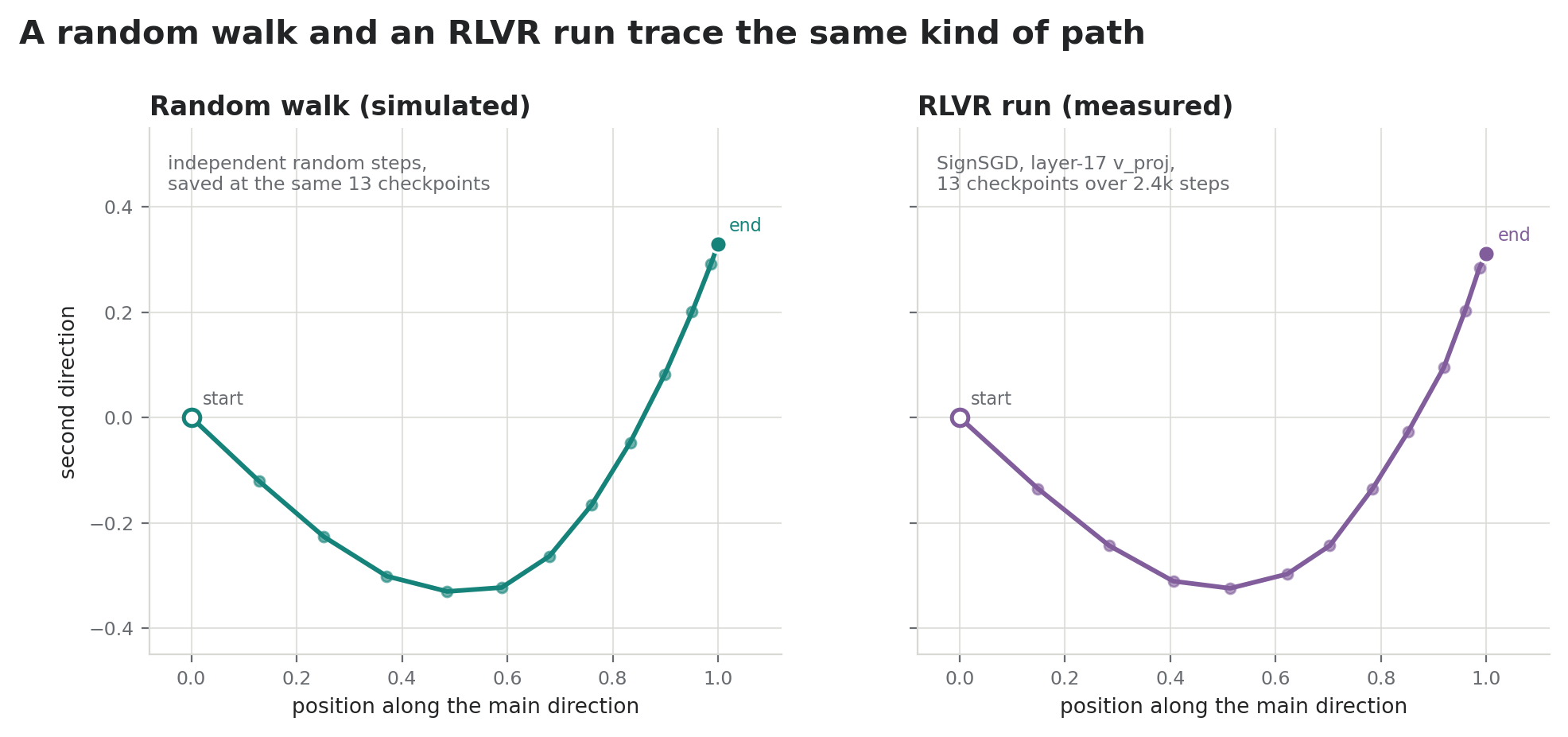
Figure 3 — A random walk and an RLVR run trace the same kind of path. Left: a simulated random walk. Right: layer 17’s v_proj update in our SignSGD run, 13 checkpoints over 2.4k steps. Each path is plotted along its own two main directions, oriented the same way and scaled so the last checkpoint sits at 1.

The weights aren’t a pure random walk either. Most tests turn up a small but systematic excess over the random walk, far too weak to extrapolate on.

2. RLVR Updates and Trajectories Are Low Rank, but So Are Random Walks

2.1 Trajectories Are Rank-One Dominant

RELEX’s first finding is about the rank of the trajectory. Stack a weight matrix’s checkpoints in order, find the directions they spread along, and one direction holds most of the variance. That sounds like a strong regularity, but every random walk has it too: with evenly spaced checkpoints, its first direction holds 81.1% of the variance.

Our runs match a random walk direction by direction (Table 1). AdamW’s first direction holds less than SignSGD’s only because its checkpoints are denser early in training (every 5 steps for the first 860 steps, then every 20), and a random walk saved at those times drops by the same amount. The second, third and fourth directions match too, and they matter as much as the first: a single number could agree by coincidence, but the whole spectrum is a fingerprint of how the trajectory was made.

Table 1 — Share of the trajectory’s variance along each of its first four directions. Full update, 42 matrices from six layers, every checkpoint (SignSGD: steps 19–2379, 119 checkpoints; AdamW: steps 4–1739, 216 checkpoints at 5- then 20-step spacing). The random walk is sampled at each run’s own checkpoint times.

The measured first direction sits slightly above the random walk on both runs, and that small excess is real.

RELEX’s own trajectory is no more concentrated than a random walk’s: within the top five directions it reports 81.4, 10.3, 4.2, 2.5 and 1.6% of the variance, against 84.5, 9.4, 3.4, 1.7 and 1.0% for a random walk.

RELEX’s first finding has a second half: rebuilding each checkpoint from the first direction alone keeps nearly all of the accuracy gain. That reproduces on our runs too, but the direction is fitted on every checkpoint up to the one being rebuilt. Section 3 separates that reconstruction from a prediction.

A Near-Linear Coefficient Inside the Window (RELEX Finding 2)

RELEX’s second finding is what makes extrapolation look safe. Take the first direction, measure how far along it each checkpoint sits (its coefficient), and the coefficient grows almost linearly with the training step. RELEX cites this as the justification for extending the line.

Our runs show the same near-linear growth. Over the whole run, a line fits the first direction’s coefficient with $R^2=0.96$ on SignSGD and 0.90 on AdamW, and a random walk gives 0.958. The line is fitted to the same checkpoints the direction was estimated from, and inside that window the coefficient simply traces the first direction’s time course. For a random walk that is a quarter sine (derived in the note above), which rises almost linearly and flattens only near the end. That is enough for a high $R^2$, even though nothing in a random walk persists from one step to the next.

RELEX reports $R^2>0.98$ for most tensors of Qwen2.5-Math-1.5B, which we did not test. On its released Qwen3-4B and Qwen3-8B checkpoints, our reimplementation gives medians of 0.90 and 0.85.²

A high $R^2$ inside the window says nothing about what the coefficient does after it. Only checkpoints held out from the fit can test that, which Section 3.3 does.

2.2 Endpoints Are Low Rank

AlphaRL’s first property is about the rank of the update: the total change to each weight matrix is dominated by a few directions. That reproduces on our runs. A convenient measure is the stable rank, which counts how many directions carry real weight:

where $\sigma_1\ge\sigma_2\ge\dots$ are the singular values of $\Delta W$. It is 1 for an update along a single direction and grows as the update spreads over more. For the full update over 2.6k steps it is about 10 for v_proj and 19 for down_proj on SignSGD, and 7 and 13 on AdamW, in matrices with 1,024 and 2,560 rows. Keeping each matrix’s top 256 directions keeps essentially all of the accuracy gain (Table 2). The stronger form of the property, that the top direction alone recovers over 99% of the gain, does not hold on our longer runs, where it keeps 39% (Section 3.1 tests AlphaRL’s rescaled version).

Table 2 — Accuracy gain kept by truncating the final update. Each matrix’s full update $\Delta W = W_{2599} - W_{19}$ is truncated to its leading singular directions, without rescaling. AIME24 avg@16 at 16k tokens, as a share of the untruncated update’s gain.

Low rank on its own doesn’t make the path predictable, though. A random walk whose steps all stay inside a small subspace ends up low rank too. Within the subspace every step still goes in a random direction, so the walk’s top direction keeps shifting, and early checkpoints say nothing about where it will point later.

Smooth Trajectories and PLS $R^2$ (AlphaRL Property 2)

AlphaRL’s second property is that the top direction moves along a nearly straight path, in step with accuracy. The paper gives two pieces of evidence, and a random walk produces both.

The first is a picture. Projected to two dimensions, the top direction at successive checkpoints traces a smooth path whose color follows training progress, which the paper reads as “a stable update direction”. An accumulated random walk traces the same kind of smooth, time-ordered path (Figure 3), a property of random walks that was known well before this debate [3]. Several of AlphaRL’s own appendix panels (Figures 16–28) are not smooth at all and show long back-and-forth jumps.

The second is a number. AlphaRL regresses checkpoint accuracy on the top direction $u_1(t)$ with one-component partial least squares (PLS), a linear fit that first compresses the thousands of coordinates of $u_1$ into a single score, and reports an average $R^2$ of 0.914. This test is easy to pass. The fit is scored on the same 27 or so checkpoints it was fitted to, and with 1,000 to 12,000 coordinates it can match almost any sequence of 27 numbers. On random directions unrelated to accuracy, it returns a median $R^2$ of 0.978 to 0.998. The paper also reports no time-only baseline, although accuracy and $u_1$ both change with training. On an accuracy curve shaped like AlphaRL’s, the training step alone, on a log scale, reaches $R^2=0.90$.

2.3 Steps Show No Persistent Direction

The tests so far look at the accumulated trajectory. A more direct test measures how far the weights move over windows of $L$ steps, averaged over every pair of checkpoints that far apart and pooled over the same 42 matrices:

The exponent says how the steps add up. If every step pointed the same way, $L$ steps of size $s$ would cover a distance $Ls$, so $\alpha=1$. If the steps point in independent random directions, they are nearly perpendicular in high dimensions and their squared lengths add, as with the sides of a right triangle: $L$ steps of size $\sigma$ cover about $\sqrt{L}\,\sigma$, so $\alpha=1/2$. That is diffusion. A small persistent part on top of the noise would bend the slope upward, toward 1, over long windows.

SignSGD diffuses at every window length we measured, and for every type of weight matrix (Figure 4). AdamW’s slope is steeper over short windows.

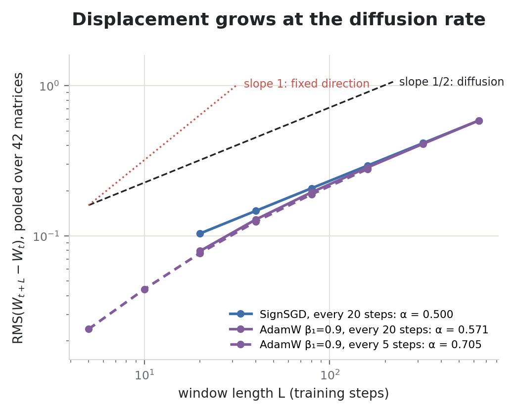
Figure 4 — Displacement grows at the diffusion rate. RMS distance moved over windows of 1 to 32 checkpoint intervals, on log axes; the legend gives each fitted slope $\alpha$. Reference slopes: 1/2 (diffusion) and 1 (a fixed direction).

Momentum explains the difference. With $\beta_1=0.9$, each step averages the gradients of roughly the last 10 steps, so neighboring steps point in similar directions and partly add end to end. Over longer windows they are independent again: AdamW’s slope falls from 0.88 between 5 and 10 steps to 0.52 between 320 and 640. A persistent direction would do the opposite and push the slope toward 1 as the windows get longer.

3. The Rank-One Direction Reconstructs Well but Predicts Poorly

We now test prediction directly, with rank-one models that see less and less of the endpoint they are trying to reach:

1. direction and distance both taken from the endpoint, which is reconstruction rather than prediction (Section 3.1);
2. direction taken from the first 100 steps, distance still taken from the endpoint (Section 3.2);
3. direction and distance both extrapolated from the first 100 steps, which is RELEX’s method (Section 3.3).

The more of the endpoint a model sees, the better it does, and only the first rung recovers the whole gain.

3.1 Fitted on the Endpoint, One Direction Reconstructs the Gain

We fix one starting checkpoint (step 19) and take four endpoints from the same run: steps 259, 499, 999 and 2,599. For each endpoint we build three rank-one models from the endpoint’s own update and ask how much of its accuracy gain each keeps:

• RELEX’s in-sample model, $W_0+\langle\Delta W,u_T\rangle\,u_T$, where $u_T$ is the trajectory’s leading direction fitted on every checkpoint up to the endpoint;
• the plain rank-one model, $W_0+\sigma_1u_1v_1^\top$, which keeps only the top singular component of each matrix’s update $\Delta W=W_T-W_0=\sum_i\sigma_iu_iv_i^\top$ (the rank of the update from Section 2.2);
• AlphaRL’s rank-one model, $W_0+\alpha\,\sigma_1u_1v_1^\top$ with $\alpha=\lVert\Delta W\rVert_F/\sigma_1$, the same component scaled up to the size of the whole update.³

Table 3 — Rank-1 recovery against training length. One starting checkpoint (step 19) and four endpoints on each run. AIME24 avg@16 at 32k; recovery of each endpoint’s own gain, with the cap-hit rate for AlphaRL’s model in parentheses. Negative values mean the model scores below the starting checkpoint. With 30 problems, the 95% intervals on these ratios span tens to hundreds of points, so we omit them. At step 2,599 the plain rank-1 model is Table 2’s rank-1 model; Table 2 scores it at 16k and against the untruncated update’s gain.

RELEX’s in-sample model reconstructs the gain at every length from step 499 on, where the gain is large enough to measure. A random walk would do the same. Projected onto its own leading direction, a random walk keeps a cosine of about 0.9 with its endpoint, because the direction was fitted with the endpoint in view. RELEX’s Finding 1 reproduces, as a reconstruction of an endpoint the direction has already seen.

The plain top direction of the update keeps a minority of the gain at every length, and only SignSGD at step 2,599 is clearly above zero. AlphaRL’s rescaled model changes with training length. On our runs the top component holds only 16–24% of the update’s norm (about 19% in AlphaRL’s own Table 7), so $\alpha$ is between four and six. At the shortest length, step 259, the rescaled model is within noise of the full gain, in line with AlphaRL’s results. As training runs longer it breaks: it soon scores below the starting checkpoint, and at step 2,599 it scores 0% on both runs, with nearly every response running into the generation cap. Its direction comes from the endpoint, but its size is extrapolated, and Section 3.3 shows what extrapolated sizes do.

Two cautions for reading Table 3. At step 259 the gain itself is small, barely distinguishable from zero on AdamW, so recoveries there are especially noisy. AdamW’s step-2,599 checkpoint scores below its step-999 checkpoint, which inflates that row’s ratios.

3.2 An Early Direction Recovers Only What Its Window Learned

The first real prediction takes the direction from early checkpoints only. Write $\Delta_t=W_t-W_0$ for the update after $t$ steps, and $u_e$ for the leading direction of the trajectory over the first $t_e$ steps, RELEX’s estimator. How much of the endpoint that direction points at is its capture:

For a random walk, the answer follows from Section 2. Steps taken after $t_e$ are nearly perpendicular to $u_e$, so the endpoint’s component along $u_e$ stays at roughly what had built up by $t_e$, while the endpoint’s length keeps growing as $\sqrt{T}$. Capture therefore falls roughly as $\sqrt{t_e/T}$. A persistent direction would keep it near 1.

Our runs follow the random walk at every window (Figure 5). SignSGD sits slightly above it throughout. AdamW’s shortest window carries some extra structure from momentum, and from 200 steps on it sits at or below the random walk. RELEX’s own held-out comparison, in its Appendix B, decays the same way (Figure 5C). A drift of 5% of the per-step noise would lift it visibly, and its numbers leave room for at most about 2%.

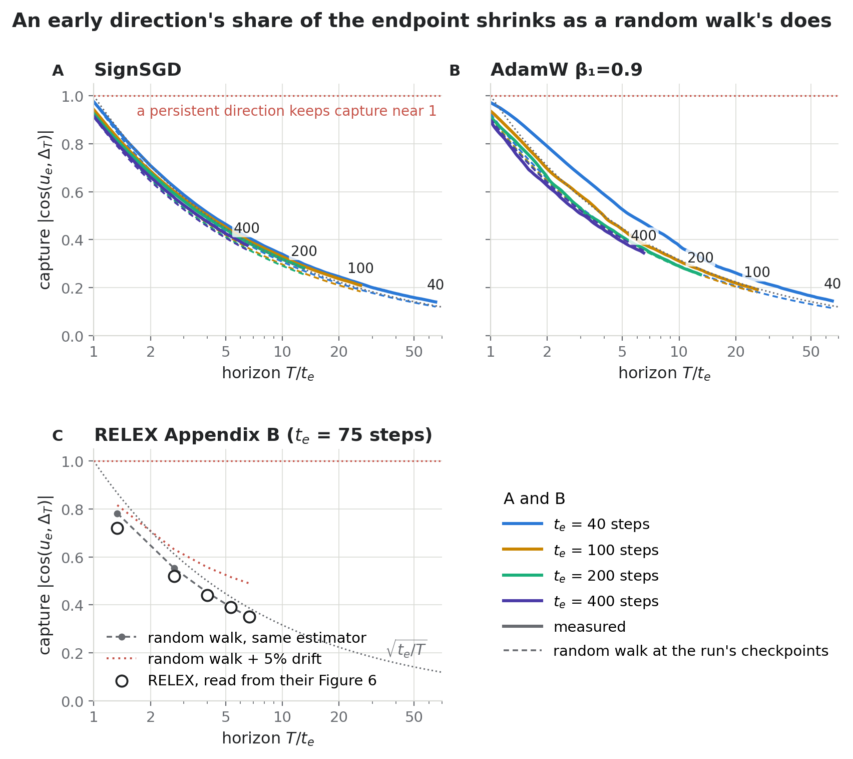
Figure 5 — An early direction’s share of the endpoint shrinks with the horizon. Capture of each later checkpoint by the leading direction of the first $t_e$ steps, against the horizon $T/t_e$. Solid: measured (42 matrices, energy-weighted); dashed: a random walk sampled at the run’s own checkpoints; dotted grey: $\sqrt{t_e/T}$; dotted red: a persistent direction. Panel C: RELEX’s held-out comparison, read from their Appendix B.

AlphaRL’s results show the same horizon effect. On DAPO with Qwen3-8B, extrapolating from 40% of training closes nearly the whole gap to full training; from 10%, less than half. At 40%, even a random walk’s early direction captures about $\sqrt{0.4}\approx0.63$ of the endpoint.

The accuracy tests that follow predict step 2,379 on SignSGD and step 1,739 on AdamW, the end of the trajectory window in Table 1. At the endpoint’s true distance, the direction from the first 100 steps recovers no detectable gain. The SignSGD model gains 2.9 points on AIME24 (95% interval [−1.3, +7.7]) against 18.5 for full training, and the AdamW model stays within noise of its base (Table 4, second row). It still lengthens AdamW’s responses toward the trained model’s, so it carries some of what the model learned in the window.

Moving the target in to RELEX’s horizons, 5 and 10 times the window, doesn’t change this (Table 5, in the collapsible note in Section 3.3). A longer window does better: the direction of the first 400 steps, moved by the true distance, keeps a significant share of the gain at a 5× horizon on both runs. That share is a little less than what training had already gained by step 400, as the random-walk argument above predicts. The endpoint’s component along an early direction is roughly what had built up by the end of the window, so the direction gives back what the window learned and nothing after it.

3.3 Extrapolating Both the Direction and Distance Causes Overshooting

RELEX’s method extrapolates the distance as well: it fits a line $c(t)=at+b$ to the coefficient $c(t)=\langle\Delta_t,u_e\rangle$ inside the early window and evaluates the line at $T$. Extending the fitted line to the endpoint overshoots the coefficient’s actual value there by 19.5× on SignSGD and 10.9× on AdamW, with the direction again taken from the first 100 steps. A random walk with the same estimator overshoots by 21× and 16×, roughly the ratio of the horizon to the window, because its coefficient levels off after the window while the line keeps climbing. AdamW overshoots less than a random walk, so its coefficient keeps growing a little after the window.

Table 4 walks the AdamW model from the true distance to the extrapolated one.

Table 4 — The extrapolation sweep on the AdamW $\beta_1=0.9$ run. The base checkpoint is step 4, the direction comes from steps 4–104, and the trained endpoint is step 1,739. AIME24 avg@16, 30k-token generation cap in a 32k context. With 30 problems, the 95% paired intervals on these differences span roughly 8 to 20 points, so we omit them; only the trained endpoint and the rows at 0.7 and 1.0 of the extrapolated scale differ significantly from the base.

No distance along this sweep improves detectably on the base model. Further out the loss becomes significant, and at the extrapolated distance itself AIME24 accuracy is 0%, with every response running into the generation cap. The failure shows up in response length first: the median response reaches the cap somewhere between 20% and 35% of the distance, before accuracy drops, and the sweep is too coarse to place the transition more precisely. Accuracy alone would miss the warning, which is why we report length and cap-hit rate next to it. AlphaRL’s rescaled model in Section 3.1 fails the same way.

About 20 times the window is further than RELEX goes: its main results extrapolate five to seven times. At that horizon the line still fails on our runs (Table 5, in the note below). Its overshoot shrinks with the horizon, to about four times at a 5× horizon, as a random walk predicted before we evaluated any model, and that is still far enough to keep no detectable share of the gain.

Nor does a window that holds more of the gain rescue the line. RELEX’s windows do: its models have three quarters of their MATH gain by step 100. From a 400-step window, which had already made about half of the target’s gain, the line and even half of it drive both runs to about 0%, with nearly every response running into the cap. Only one extrapolated model we built gains significantly: half the line from the 100-step window, on SignSGD, at a 5× horizon. A moderate push along the early direction can help a little, but the fitted line doesn’t find that distance.

On RELEX’s own recipes, extrapolation does keep the gain over moderate horizons: up to step 500, the length of its RLVR runs, every observation window keeps all three of its models near their trained MATH accuracy. Further out, only Qwen2.5-Math holds up for every window. Qwen3-8B holds with a long window but collapses with a short one (observed for 50 steps, it peaks at 86.2% at step 400 and falls to 22.7% at step 1000), and no window in the sweep holds Qwen3-4B’s accuracy beyond step 750.

The geometry doesn’t explain why RELEX’s extrapolation works and ours doesn’t. RELEX’s own line drifts as ours does (Figure 5C): on Qwen2.5-Math, extended from 75 steps to step 500, its update is 2.7 times as long as training’s and points in a quite different direction (cosine similarity 0.35), yet it matches the trained model’s MATH accuracy. It doesn’t predict the trained weights; it lands on a different model that scores as well. We suspect RELEX’s predictability comes from its particular choice of model and data combination.

4. Conclusion

Rank one was never the surprising part. A measurement is evidence for a claim only if it would come out differently were the claim false. The low-rank measurements behind predictability don’t: they hold up on our runs, but random walks produce them too, and random walks can’t be predicted.

The extrapolations in both papers work on their own recipes within limited horizons. On our runs they don’t, even at RELEX’s horizon. A direction fitted on an early window gives back about what the model had learned by the end of that window, and extending the line past it adds nothing detectable; far enough out, responses stop ending.

None of this means RLVR updates are random walks, only that these measurements can’t tell the two apart. In most tests our runs sit slightly above the random walk (Sections 2.1, 3.2 and 3.3), a small but systematic excess that is far too weak to extrapolate on.

References

[1] Zhepei Wei, Xinyu Zhu, Wei-Lin Chen, Chengsong Huang, Jiaxin Huang, Yu Meng. “You Only Need Minimal RLVR Training: Extrapolating LLMs via Rank-1 Trajectories.” University of Virginia / WashU, May 2026. RELEX.

[2] Yuchen Cai, Ding Cao, Xin Xu, et al. “On Predictability of Reinforcement Learning Dynamics for Large Language Models.” USTC / NUS / HKUST, ICLR 2026. AlphaRL.

[3] Joseph M. Antognini, Jascha Sohl-Dickstein. “PCA of High Dimensional Random Walks with Comparison to Neural Network Training.” NeurIPS 2018.