Signal or Noise? An SNR Criterion for Trusting Your Importance Ratio
Your importance ratio is a measurement, and like any measurement it contains signal (genuine policy movement) and noise from how two engines evaluate the same weights. That noise is heavy-tailed, architecturally amplified, and aimed at exactly the tokens where the learning signal lives. Guards keyed on that ratio then edit gradients on tokens whose policy never moved. We show the noise’s structure and give a procedure to measure your own signal-to-noise ratio. What that measurement licenses is the rest: how far to trust the ratio as a weight, where to bound it, and which knob to recalibrate on a factored stack. What it never licenses is letting the ratio decide which tokens to delete.
1. The Two Sides of the Importance Sampling Ratio
Truncated importance sampling and its variants have become default-on machinery across RL frameworks for off-policy correction. It is not guaranteed to save every run, though, and the published verdicts do not agree:
- Flash-RL [1] claims it enables FP8 rollouts.
- Jet-RL [2] calls the same fix “very fragile,” collapsing on long rollouts and hard tasks.
- QuRL [3] runs it out to 1600 steps and shows that the TIS corrected run finished short of the full-precision baseline it was meant to recover.
Where along the axes of context length, task difficulty, and training horizon does TIS start to break?
Instead of giving a catalog of configuration combinations, we believe the answer lies in an unmeasured quantity: the signal-to-noise ratio of the importance ratio itself.
Write the observed per-token log-ratio as the sum of two quantities with entirely different characters:
\[\log r_t \;=\; \underbrace{\alpha_t}_{\text{policy movement}} \;+\; \underbrace{\beta_t}_{\text{evaluation noise}}\]Signal and Noise Components
α is signal. It is the log-ratio between the training policy and the policy that actually sampled the token, and it goes nonzero whenever gradient updates separate the two: asynchronous staleness and multiple optimizer steps per rollout batch. These are the weight-difference sources catalogued in Off-Policy Corrections in LLM RL Training [4]. α is what importance sampling and trust-region machinery were designed for: if the policy has genuinely moved, the token’s gradient should be reweighted or bounded accordingly.
β is noise. It is what remains with bit-identical weights. The two log-probabilities are computed by different engines: different kernels and reduction orders, different discrete choices (expert routing, cached-KV versus recomputed context). These are the operator-difference families of A Field Guide to Training–Inference Corrections [5]. β is not a sampling-distribution error. The sampler really did sample from its own distribution; β is measurement error on the ratio.
A boundary case: quantized rollout
When the sampler holds lower precision version of your trainer’s weights, is it still evaluating your policy? $Q(\theta)$ is a deterministic function of $\theta$, its rounding error reaches the logits mean-zero to first order, and the bookkeeping identity of §3 pins at 1 either way. By those tests, rounding the weights is no more a change of policy than rounding the accumulator, which lands it in the $\beta$ category.
However, when the model is updated, quantization effects are coupled with the optimization process – which sets it apart from reduction order differences. Quantization has a deadband effect: an update smaller than half a cell moves $\theta$ and leaves $Q(\theta)$ where it was. RL updates routinely sit orders of magnitude below the grid, so the sampler lags the trainer and the gap widens as training runs. QuRL [3] measures that widening, with behavior-versus-proximal KL climbing from 0.002 to 0.025. Quantization here behaves similarly to staleness, which lies in the $\alpha$ category.
Ratio-conditioned interventions (importance weighting, TIS truncation, PPO-style clipping, hard rejection) apply to $\alpha + \beta$ while they were often derived under the view of pure $\alpha$.
When the observation is mostly noise, phantom clipping occurs [6]. It names a boundary decision driven by something the movement ratio should be independent of: the token’s policy never moved, and the guard edits its gradient anyway.
TRL’s precision study [6] measured it with gradient cosine, the alignment between the update a mismatched stack computes and the update the same batch would produce with no mismatch. Raw gradients score 0.95; clipped gradients fall to 0.55. Clipping itself is what misaligns the gradient direction.
Bookkeeping Decides the Mix
Which quantity your framework logs fixes the α/β composition of everything downstream. Here’s a list of common configurations:
Table 1 — Which ratio did you measure?
| numerator / denominator | engines | weight versions | content |
|---|---|---|---|
| $\pi_{\text{learner}}(\theta) \,/\, \pi_{\text{learner}}(\theta_{\text{old}})$ (PPO ratio) | same | different | α (within-rollout update drift) + β′ (within-engine noise) |
| $\pi_{\text{learner}}(\theta_k) \,/\, \pi_{\text{learner}}(\theta_j)$ (staleness ratio) | same | different | α (async staleness) + β′ |
| $\pi_{\text{learner}}(\theta_{\text{old}}) \,/\, \pi_{\text{sampler}}(\theta_{\text{old}})$ (TIS ratio) | different | same | pure β |
| $\pi_{\text{learner}}(\theta) \,/\, \pi_{\text{sampler}}(\theta_{\text{old}})$ (combined behavior ratio) | different | different | α + β mixed |
β is the cross-engine noise, and β′ is a within-engine noise term. β′ exists because of operator differences in batch size; it is typically much smaller than the cross-engine difference.
A synchronous training stack that decomposes hands its trust region a same-engine ratio that genuinely starts at 1 (row 1) and hands its mismatch machinery pure noise (row 3). A stack that does not decompose trains on row 4 and hands its machinery a sum.
The original TIS method [1] set the training–inference factor (row 3) apart from the established PPO ratio (row 1), so the trust region operates on a ratio that genuinely starts at 1. That factoring is precise, and row 3 is the consequence: with bit-identical weights on both sides, the training–inference ratio contains no policy movement at all. It is pure β by construction. The field isolated the noise into its own factor, correctly. Then it handed that isolated noise to importance-sampling machinery, as if it were a distribution shift to be corrected rather than a measurement error to be budgeted.
Table 2 — Where each component comes from, and what it scales with.
| sources | scales with | |
|---|---|---|
| α (signal) | multiple updates per rollout batch (mini-batch splits — no data reuse needed; epoch-style reuse multiplies it); async staleness; quantized-rollout lag; on-policy distillation gaps | learning rate × update count; staleness bound; update size vs quantization grid |
| β (noise) | kernel/reduction-order differences; precision (BF16 asymmetries; quantization noise at fixed weights); discrete flips (MoE routing, sparse-attention indices); cached-KV vs recomputed context | context length (accumulation); token entropy (§2); engine pair; correction config |
Shrink First, Then Measure What Survives
Before reaching for any correction mechanism, shrink what you can. Every β component you eliminate cleans the ratio for every downstream consumer: the trust region, the staleness correction, your monitoring. The toolbox is its own post [5]: specified divergences reconstructed exactly or honored by construction, discrete selections replayed or pinned, arithmetic path differences unified away, each at its own price.
What survives the toolbox is our subject. Define, per token population or per confidence bin,
\[\text{SNR} \;=\; \frac{\mathrm{Var}(\alpha)}{\mathrm{Var}(\beta)}.\]The SNR is a property of your stack, not of your algorithm. When SNR is high, the observed ratio is a trustworthy reading of policy movement, and the textbook machinery, clipping included, does what it was designed to do. When SNR is low, the same machinery is processing noise with full confidence, and every hard decision it makes is a decision made about β.
What follows:
- §2: the structure of the residual noise, and why it lands exactly where RL can least afford it.
- §3: the procedure for measuring your own split.
- §4: what the measurement licenses, which weights to trust, where to draw the bounds, and which knob to recalibrate on a factored stack.
2. The Structure of the Noise
The residual β is not the evenly distributed Gaussian noise a variance budget would assume. We find several patterns instead.
Our stack’s configuration. We measure the combined behavior ratio, row 4 of Table 1, which folds async staleness and the training–inference mismatch into a single number.1 That is why the split has to be recovered by measurement rather than read off the bookkeeping: the frozen-weight calibration below isolates β deliberately, and §3 subtracts it back out of the live ratio.
Noise is Concentrated in the Tail
To see β alone, freeze everything that could produce α: identical weights on both engines, no updates between sampling and scoring.
Table 3 — The frozen-weights $\lvert\Delta\log\pi\rvert$ distribution (identical weights on both engines).2
| statistic | value (nats) |
|---|---|
| median | 0.00015 |
| mean | 0.033 |
| p99 | 0.54 |
| max | 7.06 |
The mean is the least representative number here. The median sits two hundred times below it, and 48% of tokens agree to better than 10⁻⁴. Meanwhile the worst token is off by 7 nats. Ranked by $\lvert\Delta\rvert$, the top 1% of tokens carry 30% of the total mass, and the top 10% carry 80%.
That shape rules out the two boring explanations at a glance. Uniform numerical noise would drag the median up alongside the mean; a systematic engine offset would move the median off zero. Neither happens. β is a property of a small minority of tokens, and everything downstream depends on which minority.
The Token-Wise Amplifier
Mismatch is largest at low-probability tokens. Binned by $p_t$, our mean $\lvert\Delta\rvert$ runs monotonically from 0.00025 at $p_t > 0.99$ to 0.284 at $p_t < 0.1$, a factor of ~1100 across the confidence axis. The 8.6% of tokens with $p_t < 0.3$ carry 54% of all $\Delta$ mass; the correlation between confidence and $\lvert\Delta\rvert$ is −0.50. ByteDance’s collapse post-mortem [7] reports the same shape on a different stack.
The mechanism is the softmax. Model the accumulated numerics as a small perturbation $\varepsilon_j$, variance $\sigma^2$, on each logit. For the sampled token, $\Delta \log \pi_t = \varepsilon_t - \sum_j p_j \varepsilon_j$, which gives
\[\mathrm{Var}(\Delta \log \pi_t) \;\approx\; \sigma^2\,(1 - 2p_t + \lVert p\rVert^2).\]At a confident token, $p_t \to 1$ and $\lVert p\rVert^2 \to 1$: the variance collapses to zero, so the noise is invisible, however large σ is. At a high-entropy token, $p_t$ is small and the mass is spread so $\lVert p\rVert^2$ is small too: the variance approaches the full $\sigma^2$, and the noise is expressed at full strength. The softmax gates how loudly the same upstream noise appears, and the gate is the model’s own confidence.3
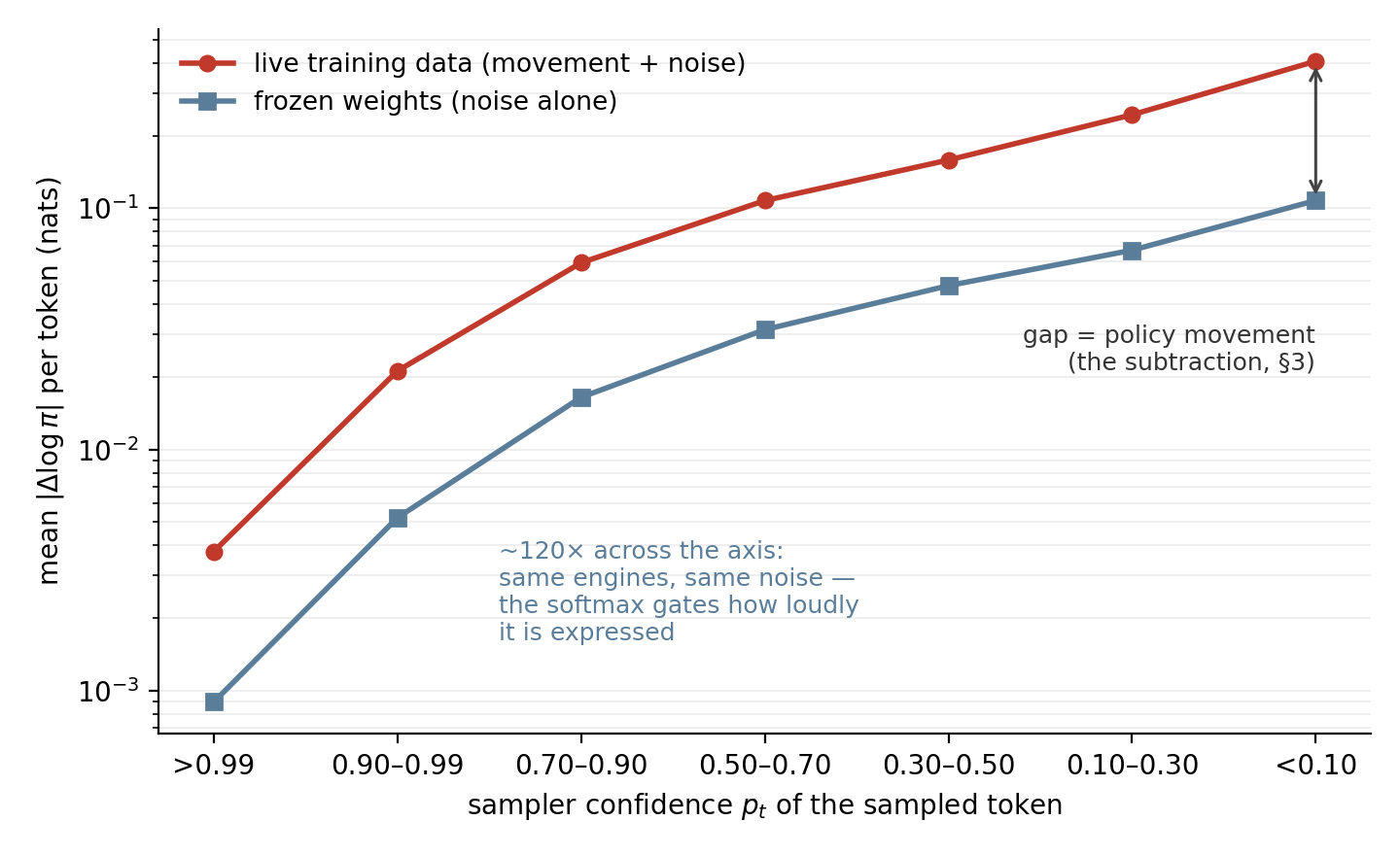
Figure 1 — The gate, measured. Mean $\lvert\Delta\log\pi\rvert$ per confidence bin under our deployed correction config (the weight-matched calibration of §3). The frozen-weights curve is β alone: same engines, same upstream noise in every bin, yet ~120× more expressed at the forks than at the confident end — the softmax gate. The live curve carries movement plus noise; the gap between the curves is what §3’s subtraction extracts.
The tail is long in absolute terms too: per-token β reaches 7 nats even at frozen weights, with noise alone producing importance ratios of $e^7 \approx 1100\times$.
The Layer-Wise Amplifier
The softmax gate explains where β is expressed, but not why σ, the accumulated logit-level perturbation, is large enough to matter in the first place. The per-operation numerical differences between two BF16 engines are tiny, fractions of a percent per layer. Why do the logits see enough noise to produce nat-scale excursions at all?
Our first answer was a hunt for a culprit. We probed one operator at a time: the output head, reduction orders, attention paths, expert compute. Each contributes only the noise you would expect from BF16 arithmetic, far too small to explain the floor. No kernel owned the mean.
What we found instead was amplification in transit. A 1% perturbation injected at layer 0 grows to 24% by mid-network: ~35× compounding, per-layer gain ≈ 1.09, saturating where the branch-input RMSNorm bounds further relative divergence. The floor is distributed, small-everywhere noise made large by the residual stream it travels through.
Why would a trained network amplify perturbations? Our conjecture is that it must: forward noise gain is the price of gradient flow. Linearize the residual stream, and a perturbation injected at layer $l$ reaches the output through $\prod_k (I + J_k)$. The gradient reaches layer $l$ through the transpose of the same product. The singular values are identical, so forward noise gain and backward gradient gain are one quantity, not two.4 A network with “stable outputs” would, by the same operator, have vanishing gradients.
Pre-norm is no special villain here. Any structure that keeps gradients alive across depth carries positive forward gain, and that is what training selects for: dynamical isometry, read in reverse. The circumstantial evidence lines up. Pre-norm holds gradients roughly constant across depth [8], and its measured forward gain compounds to match. Post-norm’s vanishing gradients dually predict noise attenuation, so the architecture the field abandoned for trainability is the one that would have suppressed the mismatch.
So the amplifier is two-stage, and it starts from per-layer numerical noise that is individually negligible:
- Residual-stream compounding: ~35× on our depth, and irreducible while the network remains trainable if the duality above holds.
- The softmax gate, $\sigma^2(1 - 2p_t + \lVert p\rVert^2)$, which aims the result at the high-entropy tokens.
What comes out is the heavy-tailed per-token β measured above. Neither stage is a bug: there was never a culprit to find. The mismatch floor is the forward shadow of gradient flow. That leaves exactly two actionable surfaces: σ itself, through the field guide’s parity and precision levers, and the decision layer that consumes the ratio.5
The Cruel Overlap: The Signal Lives in the Tail
Learning concentrates where the policy is uncertain; the amplifier expresses noise where the policy is uncertain. They are two minorities selected by the same statistic, an overlap built into the softmax by the same $1 - 2p_t + \lVert p\rVert^2$ factor.
Wang et al. [10] measured which tokens matter in RLVR: essentially all of the training signal lives in the high-entropy minority, the “forking tokens,” the ~20% of positions where the reasoning could go more than one way. Policy gradients restricted to that minority match or beat the full gradient; training on the confident majority alone degrades the model.
On our runs the fork set (bottom 20% by sampler confidence) carries 81% of all mismatch mass. Of everything a $[0.5, 2]$ rejection band touches, 89% is a fork token. β is located on the forks, so a rejection band keyed on the ratio is a near-pure fork-token deleter.
Sorting tens of millions of per-token diffs from our training runs by $\lvert\Delta\rvert$ and reading the top of the list, the worst offenders are fork tokens, by inspection: reasoning-step verbs and branch words, all at $p_t < 0.03$:
Table 4 — Worst per-token disagreements in tens of millions of live training tokens.
| token | $\lvert\Delta\log\pi\rvert$ (nats) | implied ratio | what the token decides |
|---|---|---|---|
' groups' | 7.1 | ~1160× | the object the analysis will run on |
' denote' | 4.9 | ~130× | opening a formalization |
' use' | 4.8 | ~120× | committing to an approach |
' maximum' | 3.8 | ~45× | the quantity to reason about |
'submit' (twice in the top 30) | 3.3, 3.8 | 27×, 46× | whether the solution gets graded at all |
The headline row is 'submit': the mismatch is corrupting credit assignment on the very action that earns the reward.
Other Factors that Move the Tail
Entropy. β expression is policy-conditioned, not just stack-conditioned: the gate $1 - 2p_t + \lVert p\rVert^2$ belongs to the current policy, so expressed mismatch moves whenever policy entropy moves, at fixed engine fidelity. A sharpening policy reads as improving aggregate $\lvert\Delta\rvert$ even while it dies by other means. Conversely, every entropy-raising intervention (harder data, an entropy target, a mid-run data refresh) mechanically thickens the expressed tail and the out-of-band mass.
Context length. β accumulates along the trajectory, so long-context workloads sit higher on every curve above. That is one reason the literature’s verdicts diverge along the context axis (§1).
Agentic tasks. Tool outputs are text the model never generated and is not trained on. They still push the model into unfamiliar contexts, where its next tokens come out at elevated entropy.
That is the noise: heavy-tailed, architecturally amplified, aimed at the forks, and coupled to your policy’s entropy. What none of this tells you is the split on your stack: how much of your ratio’s variance is this noise, and how much is the movement your machinery exists to handle. That is a measurement, detailed in the next section.
3. Measurements and Logging
Measuring SNR
The prerequisites, per token:
logp_sampler[t] : recorded by the rollout engine at sampling time
logp_trainer[t] : recomputed by the training engine
p_t             : trainer-side confidence of the sampled token (binning key)
Step 0 — bookkeeping sanity. The uncapped mean ratio over any large batch must pin at 1, regardless of policy movement (the identity below). If it does not: stop — you have an evaluation asymmetry, unfaithful logprobs, or a support bug.
assert mean( exp(logp_trainer - logp_sampler) ) ≈ 1 # uncapped, all tokens
For faithful per-token behavior log-probabilities, the uncapped mean ratio satisfies
\[\mathbb{E}_{a \sim \pi_{\text{sampler}}}\!\left[\frac{\pi_{\text{train}}(a)}{\pi_{\text{sampler}}(a)}\right] \;=\; \sum_a \pi_{\text{train}}(a) \;=\; 1 \qquad \text{identically.}\]On 27–31M tokens from our agentic runs it measured 1.00011 and 1.00008, so the identity holds live to four decimals.
Step 1 — calibration pass: β alone. Freeze one checkpoint θ*, load the same θ* in both engines, and generate with your deployed sampling and correction config ON (replay, masks, temperature). Corrections reshape β, so calibrate the config you actually run: enabling mask replay alone moved our fork-bin β ~1.5×. Calibrate at the weights of the live window, not at base. β grows with training: our fork-bin Var(β) at the trained checkpoint measured ~5× its base-weight value, and a base-weight calibration flattered our SNR 2–4× before we caught it.
Δ_cal[t]  = logp_trainer[t] - logp_sampler[t]      # α ≡ 0: same weights
Var_β[b]  = var( Δ_cal[t] for t with p_t in bin b )
Step 2 — live pass: α + β together. The same statistic, over ordinary training batches. Weights now differ by whatever your config produces (staleness, updates).
Δ_live[t] = logp_trainer[t] - logp_sampler[t]
Var_r[b]  = var( Δ_live[t] for t with p_t in bin b )
Step 3 — the subtraction. It assumes α and β are roughly independent within a bin, which is why the binning comes first: both components ride the entropy axis, and conditioning on the bin removes most of the shared dependence. The max(·, 0) matters too. A reading pinned at ≈0 is what a truly isolated engine-mismatch factor returns (the justification for the last row of §4’s table), so do not read it as a failed measurement. Do not assume it is what your folded ratio will return. Ours didn’t, as below.
Var_α[b]  = max( Var_r[b] - Var_β[b], 0 )          # signal variance
SNR[b]    = Var_α[b] / Var_β[b]
λ[b]      = SNR[b] / (1 + SNR[b])                  # shrinkage lookup (§4)
Refresh. β moves as training moves (§2), so redo Step 1 on a checkpoint cadence. If Var_α grows, whether from a config change, more updates per rollout, or looser staleness, then λ rises and ratio-conditioning re-engages on its own. The correction adapts to its own justification.
Run on our own stack, the procedure returns Table 5. The setup: one frozen calibration batch generated under the deployed config (mask replay and routing replay on), recomputed on the trainer at the same trained checkpoint the live window sits at. That makes α ≡ 0 by construction, with an identity check of 1.0002. We compare it against live variance from four healthy steps of an agentic run (39M masked tokens, identity 1.0002).
Table 5 — The procedure, run on our own stack. Weight-matched frozen calibration against four healthy live steps: per-confidence-bin variance split, SNR, and shrinkage λ.
| $p_t$ bin | Var_r (live) | Var_β (frozen) | Var_α | SNR | λ |
|---|---|---|---|---|---|
| < 0.10 (forks) | 0.704 | 0.130 | 0.574 | 4.4 | 0.82 |
| 0.10–0.30 | 0.280 | 0.038 | 0.242 | 6.5 | 0.87 |
| 0.30–0.50 | 0.123 | 0.022 | 0.101 | 4.6 | 0.82 |
| 0.50–0.70 | 0.061 | 0.009 | 0.051 | 5.5 | 0.85 |
| 0.70–0.90 | 0.025 | 0.005 | 0.021 | 4.5 | 0.82 |
| 0.90–0.99 | 0.0066 | 0.0014 | 0.0052 | 3.8 | 0.79 |
| 0.99–1.00 | 0.0002 | 0.00001 | 0.0001 | 12.1 | 0.92 |
Three readings:
- Every bin is signal-dominated. SNR runs roughly 4–6 across the axis, dipping to 3.8 in the 0.90–0.99 bin and reaching 12 in the near-deterministic top bin, where both variances are vanishingly small. The folded ratio is mostly α.
- Var_α is fork-concentrated, at 0.574 for the forks against 0.0001 at the confident block.
- λ ≈ 0.82–0.87 everywhere. The prescription for this ratio is mostly-trust: temper, bound the tails, never delete. That is what the clamp approximates, and what §4’s harm ordering finds from the other direction.
Reading Existing Logs
Apart from the SNR measurement, most RL frameworks have built-in statistics that can serve as proxies, but they are often conflated.
Table 6 — Existing dials, and the quantity each one actually measures.
| dial | what it actually measures | alarm reading |
|---|---|---|
| uncapped mean ratio | bookkeeping fidelity — the Step-0 identity pins it at 1 | any persistent departure |
| logged / capped mean | intervention harm — the mean of the weights that actually reach the loss; its deficit from 1 is the gradient mass your own guard is deleting | downward drift: the guard’s editing is growing |
| clip / out-of-band rate | harm token count — how many tokens the guard is touching | balloon: the tail is migrating into the band; a healthy clip rate is <1% |
| mean abs logprob diff | entropy-conflated severity — no identity anchor, and β expresses through the entropy gate, so the aggregate mixes true mismatch with batch composition | uninterpretable in aggregate; read per confidence bin only |
| sequence ESS of the IS weights | effective batch size — how many trajectories the weighted update rests on | corroborates the out-of-band rate; useful when using sequence-level clipping |
- The capped mean is the dial we ourselves misread: ours drifted 0.994 → 0.989 and convinced us of a systematic trainer-side depression, while the uncapped mean sat pinned at 1 the whole time.
- Mean $\lvert\Delta\rvert$ is the dial with no floor under it and can be a false alarm. A batch with more high-entropy tokens reads “worse” at identical engine fidelity, so an apparent improvement can be the policy sharpening, and an apparent regression can be harder prompts.
- ESS is, in practice, a sequence-level dial. It only fires when sequence-level IS is computed and whole sequences get clipped, the regime where default settings clip ~20% of trajectories. Token-level IS at a healthy clip rate (<1%) never triggers it: with 99% of weights near 1, ESS stays pinned at ~N regardless of what the tail is doing.
4. What the Measurement Licenses
The SNR sets the weight policy; the absolute tail mass sets the boundary policy. How much to trust the ratio as a multiplier scales with how much of it is signal. Whether the ratio may ever serve as a deletion key is governed by how much mass sits outside any band you draw.
The Criterion
Table 7 — The criterion. SNR of the measured ratio → correct handling.
| SNR of the measured ratio | the ratio mostly is | correct handling | where you meet it |
|---|---|---|---|
| ∞ (true parity) | signal | trust $r$; PPO-style clipping fully justified | the textbook idealization |
| high (≳ 10, because β is small) | signal, thin noise tails | standard TIS/clip semantics hold, one-sided clipping works | the benign regime: short context, non-agentic, sync or mild staleness (typical on-sync non-agentic runs) |
| moderate (our agentic runs: 4–6, with fat absolute tails) | signal-dominated mixture | trust the weight (full or lightly clamped $r$); clamp, not delete | our folded async agentic ratio (λ ≈ 0.85, Table 5): two-sided rejection collapsed the run; the same band as a clamp survived |
| ~ 1 | an even mixture — usually a config-level backend mismatch inflating β to the signal’s scale | review your stack first: config-level β should be removed, not weighted; for the residue, attenuation by $r^{\lambda}$ | trainer/sampler config divergences: TRL’s precision gap (SNR < 1 through early training) [6]; a sparsity-budget mismatch when running sparse attention |
| ≈ 0 | noise | never delete on the ratio; clamp the tails; weight ≡ 1 is the α = 0 idealization | isolated training–inference factors (pure β by construction) |
A run that survives under standard TIS may still be paying an unmeasured performance tax.
Two published counterfactuals price that tax, from different directions
- XoRL [11] prices it at a fixed horizon. On Wordle, its clamp-corrected run reaches 72.5% held-out solve rate, well above unclipped importance sampling at 63.9%, but the bitwise-identical run reaches 77.4%. The correction recovers most of the gap, and the last five points are invisible unless you run the counterfactual.
- QuRL [3] prices it as it grows. Over 1600 steps of quantized-rollout training, its ladder runs naive 52.31 → TIS 53.80 → +ACR 54.79 → +UAQ 55.48, against 56.40 in full precision. The TIS-only arm’s eval curve turns down near step 1200 while QuRL’s keeps climbing.
The dials of §3 can tell you a guard is editing gradients. Only the counterfactual tells you what the editing cost.
Treatment: Never Delete on a Fat-Tailed Ratio
The moderate row’s verdict rests on our own matched pair: same codebase, same correction stack, same two-sided band. One thing changed, delete versus clamp at the boundary. The rejection arm collapsed; the clamp arm held.
The mechanism is §2’s cruel overlap closing into a loop. 89% of what the band touches is a fork token. Deleting fork gradients degrades the policy exactly where it learns, uncertainty grows, the tail thickens, and the band deletes more. We measured it in the act: deleted mass on the rejection arm escalated 4.3× across the collapse window (0.8% → 3.6% of tokens), accelerating through the crash. The clamp arm rode the same tail-thickening at 2.4× over a longer window and never collapsed.
The verdict replicates beyond our stack:
- CISPO [12] proposed the clamp.
- ScaleRL [13] found the CISPO-style clamp the best-performing loss in its controlled recipe ablation, beating clipping-style objectives on asymptotic pass rate, and adopted it in its final recipe.
- XoRL [11] found the same clamp objective the best objective-level mitigation in its parity study, well above unclipped importance sampling, though still short of eliminating the mismatch outright.
The harm ordering on a fat-tailed folded ratio, worst first: reject > trust unbounded > clamp ≥ shrink. When the out-of-band mass is thin, rejection deletes almost nothing and beats trusting raw ratios. That is how our non-agentic runs were saved at long context. As the tail thickens, the same operation turns self-amplifying: the agentic rejection arm collapsed at an escalating 1–3.6%.
Sidedness: Two-Sided Because β Is There
The original prescriptions were one-sided. PPO’s clip caps only over-correction: bound the direction the optimizer would exploit, leave the rest alone. Decoupled PPO inherits exactly that shape for its trust region [4], and the original TIS cap [1] was one-sided too. That is the geometry you choose when you believe your ratio is signal.
Practice landed elsewhere. Our own runs required two-sided bounds for stability, and the published recipes agree.
What the two-sided adopters report
- GLM-5 [14] bounds the residual two-sidedly in its long-context recipe.
- Kimi K2.5 [15] introduces its token-level band with the explicit note that, unlike PPO clipping, it binds “regardless of the sign of the advantages,” targeting “off-policy divergence amplified by discrepancies between training and inference frameworks.”
- K3 inherits the objective, and the report calls the band essential precisely for long-horizon tool use. That is the workload §2 says steers tokens into the amplifier’s high-gain region.
The decomposition explains the migration. One-sided bounds are the right geometry for signal, which is pessimism with respect to the objective. Two-sided bounds are the right geometry for noise: β is symmetric in log space, and censoring one tail of a symmetric contamination converts mean-zero jitter into systematic, noise-correlated bias. The shape of your bound is a statement about what you believe your ratio is, and every report that found the correction “must be two-sided” is confessing that its ratio carries a directionless component.
Worse, sign-conditioned clipping leaves the negative-advantage, inflated-ratio quadrant unbounded. That is the exact cell where a β excursion on a fork token lands at full weight, and tokens there never register as “clipped,” so the clip-rate dial certifies health while the open quadrant does the damage. On SAO’s stack [16], that configuration collapses within ~90 steps with the dial near zero, while their two-sided mask holds for a thousand.
For a mixed ratio the two prescriptions compose rather than conflict: in-band weights from the dominant signal (trust the weight, λ ≈ 0.85), bound geometry from the noise (two sides). The composition lands on an asymmetric two-sided cap, because the edges do different jobs. Genuine movement skews upward in ratio space while downward excursions self-attenuate, leaving the lower edge mostly policing β’s tail, so the band carries the more tolerant upper endpoint. SAO’s disclosed math band $[0.7, 6.0]$ is −0.36/+1.79 in log space, nowhere near symmetric [16]. Where exactly the two edges go has to be calibrated. The procedure follows.
Placement: Derive the Bounds, and Refresh Them
Two-sided and clamped, then. But where do the sides go? The band has three jobs, and each derives from its own dial, per confidence bin:
- Noise exclusion: the bounds must sit outside β’s bulk, so take the frozen calibration’s empirical tail quantiles.6
- Signal coverage: the bounds must pass genuine movement, so cover ±2σ_α from the live−frozen subtraction.
- Variance guard: cap the bound where the clamped-weight effective sample size would fall through its floor (measured non-binding on our runs).
Combine as $u = \min(\max(u_{\text{noise}}, u_{\text{signal}}), u_{\text{ESS}})$, and separately for the lower edge from the lower-side quantities.
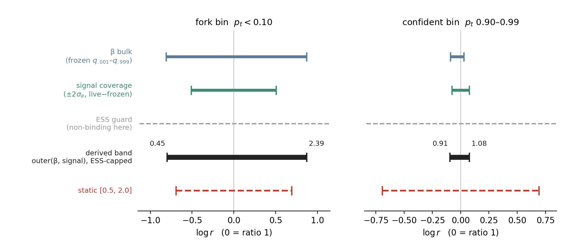
Figure 2 — The three-job rule, on two bins of one calibration. Every interval is a measured quantity (one checkpoint’s start-bound derivation). At the forks, noise exclusion binds. β’s empirical bulk reaches past the signal-coverage interval, so the derived band takes the outer envelope: $[0.45, 2.39]$, asymmetric by construction. The static $[0.5, 2.0]$ sits inside it, making noise decisions. At the confident bin the same rule returns $[0.91, 1.08]$, signal-bound at the top, and there the static band is an order of magnitude too loose in log space.
Run on our own stack, the derivation indicted the static $[0.5, 2.0]$ twice over: the fork band sat inside β’s bulk, while the confident bins were an order of magnitude too loose (Figure 2). The derived bounds also age, with the fork bound growing 2.4× in 25 iterations, so they are re-derived at checkpoint cadence and never extrapolated. When signal coverage demands bounds the variance guard forbids, treat it as a diagnosis. The ratio carries more movement than a low-variance correction can absorb: reduce the staleness or factor the ratio, don’t split the difference on the band.
Factored Ratios: Which Knob to Recalibrate
A decoupled stack guards two ratios with two knobs: a PPO clip $\epsilon$ on the movement factor, and a TIS cap $C$ on the training–inference factor. The three-job rule applies to each. The knobs are not independent, though, and that coupling is where §1’s second form of phantom clipping lives.
How a TIS cap deforms the movement band
QuRL’s objective [3] absorbs the truncation deficit into the trust region, so the effective movement band becomes $[r(1-\epsilon),\, r(1+\epsilon)]$, with $r \le 1$ the deficit on that token. Every capped token has its band re-centered below 1, and a token with no movement at all is clipped once $r < 1/(1+\epsilon)$. Nothing is flipped by noise here. The mismatch reading deterministically sets the movement guard’s geometry, which is what makes this form structural rather than stochastic.
Read that schedule against Figure 2 and it runs backwards. A larger mismatch reading means a smaller $r$, so a narrower movement band, drawn tightest on the fork tokens the derivation gives the widest one.
QuRL repairs the deformation by raising the PPO ceiling in proportion, which flattens the accidental schedule back to a constant but calibrates it to nothing measured. We would suggest recalibrating the other knob. $C$ is the term that carries the mismatch, so $C$ is the term the three-job rule should size: per-bin quantiles from the frozen calibration, with the ESS guard as its ceiling so it never chases the tail. The movement band is then left at the textbook $\epsilon$, which a near-pure-α ratio licenses on its own.
5. Conclusion
Four takeaways:
Know which ratio your machinery holds. “The” importance ratio is several different objects, and your bookkeeping fixes the α/β composition before any statistic is computed.
The noise has structure. β is heavy-tailed, gated by the softmax onto exactly the fork tokens where the learning signal lives, and moved by your corrections, your policy’s entropy, and your workload. No ratio threshold separates it from genuine movement.
- SNR sets the weight policy; tail mass sets the boundary policy. Trust the weight in proportion to λ, and never let a fat-tailed ratio serve as a deletion key. Clamp instead. The bounds themselves are derived quantities: two-sided because of β, asymmetric because of α, calibrated from the same measurement, and refreshed on cadence because every floor in this problem moves.
- Every “fine” is a floor, not a ceiling. The evidence behind the field’s verdicts, ours included, only tells you a run survived. A surviving run can still be paying a tax no dial reports.
So the question the literature has been asking — is TIS useful? does clipping help? one-sided or two? — was never a yes/no question about an algorithm. It is a measurement: of the ratio your bookkeeping produces, on your stack, under your workload, refreshed as training moves it. Verdicts age with their regimes. Measurements are what carry over.
References
[1] Feng Yao, Liyuan Liu, Dinghuai Zhang, Chengyu Dong, Jingbo Shang, Jianfeng Gao. “Your Efficient RL Framework Secretly Brings You Off-Policy RL Training.” 2025. Flash-RL.
[2] Haocheng Xi, Charlie Ruan, Peiyuan Liao, et al. “Jet-RL: Enabling On-Policy FP8 Reinforcement Learning with Unified Training and Rollout Precision Flow.” NVIDIA / MIT / UC Berkeley, January 2026.
[3] Yuhang Li, Reena Elangovan, Xin Dong, Priyadarshini Panda, Brucek Khailany. “QuRL: Efficient Reinforcement Learning with Quantized Rollout.” NVIDIA Research / Yale / USC, ICLR 2026.
[4] Off-Policy Corrections in LLM RL Training. March 2026.
[5] A Field Guide to Training–Inference Corrections. September 2026.
[6] Amine Dirhoussi, Quentin Gallouédec, Edward Beeching, Lewis Tunstall, Kashif Rasul, Leandro von Werra. “Defeating the trainer-generator precision mismatch in TRL.” Hugging Face, 2026.
[7] Jiacai Liu, Yingru Li, Yuqian Fu, Jiawei Wang, Qian Liu, Yu Shen. “When Speed Kills Stability: Demystifying RL Collapse from the Training-Inference Mismatch.” ByteDance, September 2025.
[8] Ruibin Xiong, Yunchang Yang, Di He, et al. “On Layer Normalization in the Transformer Architecture.” ICML 2020.
[9] Laker Newhouse, R. Preston Hess, Franz Cesista, Andrii Zahorodnii, Jeremy Bernstein, Phillip Isola. “Training Transformers with Enforced Lipschitz Constants.” July 2025.
[10] Shenzhi Wang, Le Yu, Chang Gao, et al. “Beyond the 80/20 Rule: High-Entropy Minority Tokens Drive Effective Reinforcement Learning for LLM Reasoning.” Qwen Team / LeapLab, June 2025.
[11] Ashwinee Panda. “0 train-infer mismatch for Open-weight MoE RL in Open-source code.” TogetherAI, 2026. XoRL.
[12] MiniMax. “MiniMax-M1: Scaling Test-Time Compute Efficiently with Lightning Attention.” June 2025.
[13] Devvrit Khatri, Lovish Madaan, Rishabh Tiwari, et al. “The Art of Scaling Reinforcement Learning Compute for LLMs.” Meta, October 2025.
[14] GLM-5 Team, Zhipu AI & Tsinghua. “GLM-5: from Vibe Coding to Agentic Engineering.” February 2026.
[15] Kimi Team. “Kimi K2.5: Visual Agentic Intelligence.” February 2026, §4.4.2.
[16] Zhenyu Hou, Yujiang Li, Jie Tang, Yuxiao Dong. “Single-Rollout Asynchronous Optimization for Agentic Reinforcement Learning.” Tsinghua / Z.AI, July 2026.
Factoring the combined ratio into a separate staleness term and training–inference term (rows 1 and 3) means holding the log-probabilities of more than one weight version. In an async stack with partial rollout, a single sequence can span several versions, so that separation requires bookkeeping multiple model versions on the training engines. We fold instead, and pay for it with the calibration pass of §3. ↩
This calibration was taken at a checkpoint on the edge of collapse, so the log-prob differences run larger than a typical healthy run’s. β grows with training (§3’s moving-floor lesson). What we use here is the distribution’s shape, meaning the concentration and the heavy tail, and that holds at every checkpoint we have measured. ↩
The derivation treats the logit perturbations $\varepsilon_j$ as independent with equal variance. In reality they arrive largely as one shared hidden-state perturbation projected through the unembedding, so they are correlated across the vocabulary. The exact $1 - 2p_t + \lVert p\rVert^2$ form is the iid idealization; what the binned measurement tests, and what holds, is the gate’s monotonicity. ↩
Exact for the singular-value spectrum: numerical noise probes random directions while gradients are loss-aligned, so the two gains share a spectrum without being numerically identical. That is why this is a conjecture, not a theorem about our floor. ↩
A third surface is emerging: enforcing Lipschitz bounds on the transformer itself, meaning weight-norm constraints that cap the network’s gain directly [9]. Unlike parity work, this attacks the compounding stage rather than the per-operation noise. It is ongoing research. The trainability price the duality predicts is real at the scales tested, and the approach has not been scaled up, so it is a lever to watch rather than one to pull. ↩
Not a place for Gaussian shortcuts: β’s heavy tail means a 3σ rule understates the fork bound by roughly 3× on our measurements. ↩