Off-Policy Corrections in LLM RL Training
Published:
A unified view of the five sources of distribution mismatch in LLM reinforcement learning and their corrections.
The Unified Problem
Every off-policy issue in LLM RL reduces to the same fundamental problem:
\(\text{We sample from } \pi_{\text{actual}} \text{ but optimize as if samples came from } \pi_{\text{assumed}}\)
When $\pi_{\text{actual}} \neq \pi_{\text{assumed}}$, the policy gradient becomes biased. The general correction is importance sampling:
Theoretical grounding [1]: The token-level optimization objective used by REINFORCE, GRPO, and related algorithms is a first-order approximation to the true sequence-level reward objective. This approximation is valid only when each token’s IS ratio $\delta_t = \frac{\pi_\theta(y_t)}{\mu_{\theta_{old}}(y_t)} - 1$ is small, so that second-order terms ($\delta_i \delta_j$) can be neglected. The token-level IS weight is therefore inherent to the approximation — not an optional correction bolted on. Removing it invalidates the surrogate objective entirely.
In LLM RL, five distinct sources create this mismatch, each with different causes, magnitudes, and corrections:
| # | Source | $\pi_{\text{actual}}$ | $\pi_{\text{assumed}}$ | Magnitude | When it arises |
|---|---|---|---|---|---|
| 1 | Multi-epoch policy drift | $\pi_{\theta_{old}}$ (start of epoch) | $\pi_\theta$ (current params) | Small per epoch | PPO/GRPO multi-epoch training |
| 2 | Backend mismatch | $\pi_{\text{sampler}}(\theta)$ (vLLM/SGLang) | $\pi_{\text{learner}}(\theta)$ (FSDP/Megatron) | Small but systematic under fp16 | Different engines for rollout vs training |
| 3 | Async staleness | $\pi_{\theta_k}$ ($k$ steps old) | $\pi_\theta$ (current) | Can be large | Async RL |
| 4 | MoE routing | $\pi_\theta$ with route_old | $\pi_\theta$ with route_new | Variable, depending on model routing stability | MoE architectures after gradient updates |
| 5 | Tool-call trajectories | $\pi_\theta \times P_{\text{env}}$ (joint) | $\pi_\theta$ (LM only) | Variable, can be large | Agentic RL with tool use |
Sources 1–3 are independent and their corrections compose cleanly. Source 4 (MoE routing) is qualitatively different — it’s a discrete structural change that amplifies Sources 2 and 3 rather than being fully independent. Source 5 (tool-call trajectories) is also qualitatively different — the mismatch comes from non-policy tokens in the conditioning context rather than from policy weight differences.
The IS Aggregation Problem: Why No Practical Method Is Exact
Before diving into individual sources, it’s worth understanding a fundamental limitation that underlies all of them.
For a sequence-level reward $R(x,y)$, the exact IS gradient requires the full product of per-token ratios:
\[\nabla_\theta J(\theta) = \mathbb{E}_{y \sim \mu_{\theta_{old}}}\left[\prod_{t=1}^{\lvert y \rvert} \frac{\pi_\theta(y_t \mid y_{<t})}{\mu_{\theta_{old}}(y_t \mid y_{<t})} \cdot R(x,y) \cdot \sum_{t} \nabla_\theta \log \pi_\theta(y_t \mid y_{<t})\right]\]The per-token ratio $\frac{\pi_\theta(y_t \mid y_{<t})}{\mu_{\theta_{old}}(y_t \mid y_{<t})}$ is the correct building block. But the product of these ratios over a full sequence is intractable — for $\lvert y \rvert = 1000$ tokens, even with each ratio in $[0.99, 1.01]$, the product ranges from $\approx 0.00004$ to $\approx 22026$. Variance grows exponentially with sequence length, making gradient estimates useless.
Every practical algorithm approximates this product differently:
| Approach | IS weight used | Relation to exact $\prod_t r_t$ | Tradeoff |
|---|---|---|---|
| Exact | $\prod_t r_t$ (full product) | Correct | Intractable variance |
| GRPO (token-level) | Per-token $r_t$ in PPO surrogate (gradients flow through) | Same first-order token-level approx: $\prod(1+\delta_t) \approx 1 + \sum \delta_t$ | Low bias when ratios $\approx$ 1; breaks down far from on-policy |
| CISPO (token-level, detached) | Per-token $\text{clip}(r_t)$ as detached weight on log-prob | Same first-order token-level approx, but ratio is clipped and stop-gradient | Preserves all tokens; slight bias from weight clipping |
| GSPO (sequence geometric mean) | $(\prod_t r_t)^{1/\vert y\vert}$ applied uniformly | $\vert y\vert$-th root of exact product — a heuristic, not a principled approximation | Low variance; unclear what bias it introduces |
The fundamental tension: sequence-level rewards demand sequence-level IS, but sequence-level IS has exponential variance in autoregressive models. There is no free lunch — every method trades bias for variance differently. The practical question is which approximation degrades most gracefully as the five mismatch sources push ratios away from 1.
Source 1: Multi-Epoch Policy Drift
What happens: PPO and GRPO reuse the same batch of rollouts for multiple gradient steps (epochs). After the first update, the policy $\pi_\theta$ has drifted from the sampling policy $\pi_{\theta_{old}}$.
Correction: The standard IS ratio with clipping, built into the algorithm:
\[r_t(\theta) = \frac{\pi_\theta(a_t \mid s_t)}{\pi_{\theta_{old}}(a_t \mid s_t)}, \quad L = \min\left(r_t A_t, \text{clip}(r_t, 1-\epsilon, 1+\epsilon) A_t\right)\]This is the most well-studied mismatch and is already handled by the algorithm’s own clipping mechanism.
Interaction with KL: When using “KL in reward” (combined form), PPO’s clipping automatically provides IS correction for the KL term. When using “KL as loss” (decoupled form), the KL term needs its own explicit IS correction across epochs — applying the same importance ratio $\rho_k(\theta) = \pi_\theta / \pi_{\theta_k}$ to the KL loss, with clipping: $\min(\rho_k \cdot k_n’,\; \text{clip}(\rho_k, 1-\epsilon, 1+\epsilon) \cdot k_n’)$. See [2] for the full analysis.
Source 2: Backend Mismatch (TIS)
What happens: In disaggregated RL systems, the rollout engine (vLLM/SGLang) and training engine (FSDP/Megatron) use different backends. Even with identical weights, these backends produce different log-probabilities due to:
- Different attention kernels (e.g., FlashAttention variants)
- Different operator fusion patterns
- Quantization differences (FP8/INT8 rollout vs BF16 training)
- Numerical precision handling (accumulated floating-point differences)
This creates an unintentional off-policy gap: $\pi_{\text{sampler}}(\theta) \neq \pi_{\text{learner}}(\theta)$.
When it arises: Whenever rollout and training use different software backends — which is the common case in both colocated and disaggregated setups. Note that “colocated” means the same GPUs are time-shared between rollout and training phases, but most colocated frameworks still use different engines (e.g., vLLM for inference, FSDP for training) on those GPUs. Backend mismatch is eliminated only when both phases use the same engine (e.g., the training framework’s own generate()), which sacrifices inference throughput significantly and is rare in practice.
Three Log-Probabilities
When backend mismatch exists, we need three distinct log-probabilities:
flowchart LR
    subgraph rollout["Rollout Phase"]
        direction TB
        P["Prompt"] --> SAM["Sampler (vLLM)"]
        SAM --> LSAM["① log π_sam(θ_old)"]
    end

    subgraph training["Training Phase — Learner (FSDP)"]
        direction TB
        FP1["③ FP#1 (θ, grads) → log π_learn(θ)"]
        FP2["② FP#2 (θ_old, no grad) → log π_learn(θ_old)"]
    end

    LSAM -- "cached" --> training
- $\log \pi_{\text{sampler}}(a, \theta_{\mathrm{old}})$ — from rollout backend at time of sampling (cached)
- $\log \pi_{\text{learner}}(a, \theta_{\mathrm{old}})$ — from training backend with $\theta_{\mathrm{old}}$ weights (FP#2, detached)
- $\log \pi_{\text{learner}}(a, \theta)$ — from training backend with current weights (FP#1, with gradients)
Correction Approach 1: Resampling
Recompute log-probs using the training backend, discarding the sampler’s log-probs entirely:
\[\frac{\pi_{\text{learner}}(a, \theta)}{\pi_{\text{learner}}(a, \theta_{\mathrm{old}})} \quad \text{(both from same backend)}\]- Pro: Same-backend ratio; no mismatch in the PPO ratio itself
- Con: Requires extra forward pass (FP#2); the expectation is still taken over $\pi_{\text{sampler}}$, so a distributional mismatch remains in the sampling distribution
- Used by: VeRL (built-in implementation)
Correction Approach 2: Truncated Importance Sampling (TIS)
Explicitly correct for the backend gap with a truncated importance ratio:
\[r_{\text{TIS}} = \min\left(\frac{\pi_{\text{learner}}(a, \theta_{\mathrm{old}})}{\pi_{\text{sampler}}(a, \theta_{\mathrm{old}})}, C\right)\]where $C$ is a loose cap (typically 10–100, much larger than PPO’s $1+\epsilon$). The full loss becomes:
\[\mathcal{L} = -\frac{1}{B \times G} \sum_{i} r_{\text{TIS}} \cdot \min\left(r_{\text{PPO}} \cdot A_i, \text{clip}(r_{\text{PPO}}, 1-\epsilon, 1+\epsilon) \cdot A_i\right)\]with two separate ratios serving distinct roles:
- $r_{\text{TIS}}$ corrects for backend mismatch (should be $\approx 1.0$ if backends are close)
- $r_{\text{PPO}} = \frac{\pi_{\text{learner}}(a, \theta)}{\pi_{\text{learner}}(a, \theta_{\mathrm{old}})}$ handles policy drift (same backend, no mismatch)
The gradient flows through $r_{\text{PPO}}$ but $r_{\text{TIS}}$ is detached (no gradient through old policy).
Why Not Combine Into a Single Ratio?
A natural idea: skip the separation and use $\frac{\pi_{\text{learner}}(a, \theta)}{\pi_{\text{sampler}}(a, \theta_{\mathrm{old}})}$ directly as the PPO ratio. This doesn’t work well in practice.
From the Flash-RL team [3]:
Even when $\theta = \theta_{\mathrm{old}}$, the probability ratio $\frac{\pi_{\mathrm{learner}}(a, \theta)}{\pi_{\mathrm{sampler}}(a, \theta_{\mathrm{old}})}$ is already not equal to 1 due to the mismatch — this makes the clipping happen with high possibility and the training much less informative. Furthermore, in our TIS method, we separately clip $\frac{\pi_{\mathrm{learner}}(a, \theta_{\mathrm{old}})}{\pi_{\mathrm{sampler}}(a, \theta_{\mathrm{old}})}$ and $\frac{\pi_{\mathrm{learner}}(a, \theta)}{\pi_{\mathrm{learner}}(a, \theta_{\mathrm{old}})}$ and thus much more mild; notice $\frac{\pi_{\mathrm{learner}}(a, \theta)}{\pi_{\mathrm{learner}}(a, \theta_{\mathrm{old}})}$ equals to 1 when $\theta = \theta_{\mathrm{old}}$ which is suitable for the trust region constraint.
The key insight: PPO’s trust region is designed around the assumption that the ratio starts at 1.0. Backend mismatch violates this assumption, causing excessive clipping and uninformative gradients. Separating the two ratios preserves the trust region semantics.
Aside: Sequence-Level Tolerance
The GSPO paper [4] claims that sequence-level likelihoods are more tolerant of backend precision differences, since small per-token numerical errors may cancel out when aggregated via the geometric mean. If true, this would let GSPO skip TIS entirely — reducing the training node to a single forward pass. However, the geometric mean is not a principled approximation to the exact sequence-level IS product (it’s the $\vert y\vert $-th root, a fundamentally different quantity). We mention it for completeness but would not rely on it as a general-purpose correction strategy.
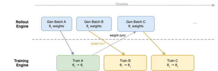
Source 3: Async Staleness
What happens: In asynchronous RL systems, the rollout engine generates data using policy weights from $k$ training steps ago ($\pi_{\theta_k}$), while the training engine optimizes the current policy ($\pi_\theta$). The staleness $k$ depends on system throughput and scheduling.
When it arises: Any system where rollout and training overlap in time:
- Fully async systems (e.g., AReaL [5], Slime async mode)
- Double-buffered / pipelined systems (generating batch N+1 while training on batch N)
- Systems with slow weight synchronization
Why it’s worse than multi-epoch drift: Multi-epoch drift is bounded (typically 1–4 epochs, each a small gradient step). Async staleness is unbounded without explicit control — the policy can drift arbitrarily far between when data was generated and when it’s consumed for training.
Prevention: Staleness Rate-Limiting
Rather than correcting stale data after the fact, bound how stale data can get:
\[\lfloor (N_r - 1) / B \rfloor \leq i + \eta\]Where:
- $N_r$ = total generated trajectories so far
- $B$ = training batch size
- $i$ = current policy version (increments each training step)
- $\eta$ = maximum staleness budget
The rollout controller blocks new generation requests when this bound is violated, unblocking when training completes a step.
Recommended values (from AReaL): $\eta = 4$ for coding tasks, $\eta = 8$ for math tasks. Tighter bounds mean less staleness but more pipeline bubbles; looser bounds improve throughput but degrade convergence.
Correction: Decoupled PPO
When data is stale, standard PPO’s trust region is misplaced — it clips around $\pi_{\theta_k}$ (the stale behavior policy) rather than the current policy. AReaL’s decoupled PPO separates two roles:
- Behavior policy $\pi_{\text{behav}}$: the (possibly stale) policy that generated the data
- Proximal policy $\pi_{\text{prox}}$: current policy snapshot, used as the trust region center
where $u_t^{\text{prox}}(\theta) = \frac{\pi_\theta(a_t \mid s_t)}{\pi_{\text{prox}}(a_t \mid s_t)}$.
The importance weight $\pi_{\text{prox}} / \pi_{\text{behav}}$ corrects for distribution shift. The clip operates around $\pi_{\text{prox}}$ (a recent, high-quality policy) rather than $\pi_{\text{behav}}$ (potentially stale).
Implementation: Store log_prob_behav during generation, tagged with the policy weight_version. Before training, compute log_prob_prox via a forward pass with the current policy snapshot.
Heuristic Corrections
Two simpler (but less principled) alternatives:
Off-Policy Sequence Masking (OPSM): Discard entire sequences whose importance ratio $\pi_\theta / \pi_{\theta_k}$ exceeds a threshold. Simple but wastes gradient signal from masked sequences.
TIS for staleness: Apply truncated importance sampling (same mechanism as Source 2) to the staleness ratio. Clips extreme ratios but doesn’t relocate the trust region.
Why Both Prevention and Correction Are Needed
AReaL’s ablations demonstrate that neither rate-limiting nor decoupled PPO alone is sufficient:
| Setup | Result |
|---|---|
| Naive PPO, $\eta$=1 | Degraded vs synchronous |
| Naive PPO, $\eta$=4 | Collapsed |
| Decoupled PPO, $\eta$=$\infty$ (unbounded) | Degraded |
| Decoupled PPO, $\eta \leq 8$ | Matches synchronous oracle |
Prevention ($\eta$) bounds worst-case staleness; correction (decoupled PPO) handles the residual drift within that bound. The combination is what makes fully async training viable.
Source 4: MoE Routing Mismatch
What happens: In Mixture-of-Experts models, the router selects which experts process each token. After a gradient update, the router’s decisions might change. This is more prominent in deeper MoE architectures.
Why it’s listed separately: Unlike Sources 1–3, this mismatch involves a discrete structural change (different experts activated) rather than continuous numerical drift. However, mechanistically, MoE routing is entangled with Sources 2 and 3 — it amplifies both backend mismatch and policy staleness.
How Routing Amplifies Sources 2 and 3
The Qwen team’s analysis [1] shows that for MoE models, the token-level IS weight decomposes as:
\[\frac{\pi_\theta(y_t \mid x, y_{<t})}{\mu_{\theta_{old}}(y_t \mid x, y_{<t})} = \underbrace{\frac{\pi_{\theta_{old}}(y_t \mid x, y_{<t}, e^{\pi}_{old,t})}{\mu_{\theta_{old}}(y_t \mid x, y_{<t}, e^{\mu}_{old,t})}}_{\text{training-inference discrepancy}} \times \underbrace{\frac{\pi_\theta(y_t \mid x, y_{<t}, e^{\pi}_t)}{\pi_{\theta_{old}}(y_t \mid x, y_{<t}, e^{\pi}_{old,t})}}_{\text{policy staleness}}\]where $e^{\pi}$ and $e^{\mu}$ denote the routed experts in the training and inference engines respectively. Expert routing now appears inside both factors:
- Training-inference discrepancy: Even with identical weights, the training engine and inference engine may route to different experts ($e^{\pi}_{old,t} \neq e^{\mu}_{old,t}$), amplifying the numerical differences that already exist from different kernels/precision.
- Policy staleness: After gradient updates, not only do the model parameters change, but the routed experts also shift $e^{\pi}_t \neq e^{\pi}_{old,t}$, compounding the distribution shift.
This entanglement is why MoE RL training is fundamentally harder to stabilize than dense model training — routing noise makes the first-order approximation break down faster.
Correction: Routing Replay
The core idea: fix the routed experts during policy optimization so the model behaves like a dense one for IS computation purposes. Two variants exist [1]:
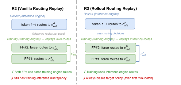
R2 (Vanilla Routing Replay): Replay the training engine’s routing ($e^{\pi}_{old,t}$). Reduces the policy staleness component. For the first mini-batch of a global step, the target policy is unaltered; for subsequent mini-batches, the forced routing deviates from the model’s natural routing, biasing the optimization target.
R3 (Rollout Routing Replay): Replay the inference engine’s routing ($e^{\mu}_{old,t}$). Reduces the training-inference discrepancy by forcing the training engine to use the same experts the inference engine chose. Always alters the target policy (even in the first mini-batch), since the training engine is forced to use the inference engine’s routing decisions.
Critical finding — R2 vs R3 depends on off-policiness:
| Off-policiness $N$ (global batch / micro-batch) | Better variant | Why |
|---|---|---|
| Small ($N$=2) | R2 | R2 preserves target policy in first mini-batch; R3’s bias outweighs its discrepancy reduction |
| Large ($N \geq 4$) | R3 | Training-inference discrepancy dominates; R3’s reduction of this factor outweighs its target-policy bias |
| Very large ($N$=8) | R3 essential | R2 fails to sustain stable training; only R3 + clipping remains viable |
On-policy training ($N$=1): Neither R2 nor R3 provides benefit — Routing Replay introduces bias without compensating gain. The basic algorithm with IS correction (no Routing Replay) achieves the best performance.
Shared drawbacks of both variants:
- Additional memory overhead (must store routing decisions per token)
- Communication overhead in distributed settings
- Introduces optimization bias by forcing non-natural expert assignments
Alternative: Sequence-Level IS (GSPO)
GSPO sidesteps routing replay entirely by operating at the sequence level using a geometric mean of per-token ratios: $s_i(\theta) = (\pi_\theta(y_i \mid x) / \pi_{\theta_{old}}(y_i \mid x))^{1/\lvert y_i \rvert}$. The intuition is that aggregating across the full sequence dilutes individual routing fluctuations, avoiding the bias that Routing Replay introduces by forcing expert assignments.
Caveats: The geometric mean is not a principled approximation to the exact sequence-level IS product — it’s a heuristic that happens to have low variance. The GSPO paper [4] demonstrates stability on Qwen3’s MoE architecture, but Qwen3 appears to have relatively stable routing behavior. Whether this generalizes to architectures with more volatile routing (deeper models, different load-balancing) is unclear. The practical benefits (no Routing Replay memory/communication overhead, no target-policy bias) are real, but they come from a theoretically unmotivated transformation of the IS ratio.
Source 5: Tool-Call Trajectory Mismatch (Agentic RL) — Emerging
Note: This source is relatively under-studied compared to Sources 1–4. Most of the analysis below is based on theoretical reasoning and early observations rather than large-scale empirical validation. We include it because it will become increasingly important as agentic training scales, but readers should calibrate their confidence accordingly.
What happens: In agentic RL training, trajectories are multi-turn with interleaved LM output and tool/environment output:
Turn 1:  LM generates action a₁ ~ π_θ(·|x)
         Tool returns observation o₁  ← NOT from π_θ
Turn 2:  LM generates action a₂ ~ π_θ(·|x, a₁, o₁)
         Tool returns observation o₂  ← NOT from π_θ
...
Tool output tokens (code execution results, search snippets, API responses) are not drawn from the LM policy — they come from the environment. While loss is not computed over tool output tokens (they are masked), they appear in the conditioning context for subsequent LM generations.
The off-policy effect: Unlike Sources 1–4, where the mismatch is between different versions or implementations of the same policy, Source 5 involves tokens from a fundamentally different generative process (the environment) appearing in the LM’s context. This has three consequences:
Distribution shift in conditioning: Tool outputs push the LM into distribution regions it would rarely visit through autoregressive generation alone. This is by design — tool use is valuable precisely because it gives the LM access to information it couldn’t generate — but it creates a challenging optimization landscape.
IS ratio instability: When the policy updates (Sources 1/3), the LM’s response to tool outputs can shift disproportionately. Tool-conditioned continuations sit in a high-sensitivity region of the distribution: small weight changes $\theta \to \theta’$ can cause large changes in $\pi_{\theta’}(a_t \mid \text{context with tool output})$. This amplifies IS ratios for post-tool tokens, leading to more clipping and less gradient signal from the most informationally rich parts of the trajectory.
Aggravated backend mismatch (Source 2): Low-probability tokens are where floating-point precision differences between backends matter most — relative numerical error is proportionally larger in the tail of the distribution. Since tool-conditioned context pushes the LM to generate tokens it otherwise wouldn’t, the log-prob discrepancy between sampler and learner backends is systematically worse on post-tool tokens.
Why standard IS doesn’t help: For Sources 1–4, the correction is conceptually clear — ratio the generating policy against the assumed policy. For Source 5, there is no “tool output policy” to ratio against. The tool outputs are fixed observations from the environment; the issue is that conditioning on them creates a more volatile optimization target, not that they were sampled from the wrong distribution.
What practitioners currently do: Masking tool output tokens from loss is standard practice. Beyond that, some apply TIS-style ratio clipping to post-tool tokens, and some frameworks compute advantages at the turn level rather than the full trajectory level.
How Corrections Compose
In production systems, multiple sources of mismatch coexist. Understanding how their corrections interact is critical.
Ratio Decomposition
For a fully async, disaggregated MoE system, the complete correction at the token level decomposes into four independent factors:
\[\underbrace{\frac{\pi_{\text{learner}}(\theta_k)}{\pi_{\text{sampler}}(\theta_k)}}_{\substack{\textbf{backend (Source 2)} \\ \text{Detached, cap } C \in [2,10] \\ \text{Eliminated if same engine}}} \;\times\; \underbrace{\frac{\pi_{\text{prox}}}{\pi_{\theta_k}}}_{\substack{\textbf{staleness (Source 3)} \\ \text{Detached (weight)} \\ \text{Eliminated if sync}}} \;\times\; \underbrace{\frac{\pi_\theta}{\pi_{\text{prox}}}}_{\substack{\textbf{trust region (Source 1)} \\ \text{Clipped } [1\!-\!\epsilon,\; 1\!+\!\epsilon] \\ \text{Always present}}} \;\times\; \underbrace{[\text{routing fix}]}_{\substack{\textbf{MoE (Source 4)} \\ \text{R2/R3 replay} \\ \text{Eliminated if dense}}}\]This is why simplifying assumptions matter: using the same engine for rollout and training eliminates the backend factor (rare in practice), synchronous training eliminates the staleness factor, and tight staleness bounds ($\eta$) keep it small.
GSPO claims to dilute factor 4 via sequence-level aggregation, though the theoretical basis for this is weak (see Source 4 caveats).
TIS × Multi-Epoch (Disaggregated PPO/GRPO)
The most common combination. The full loss:
\[\mathcal{L} = r_{\text{TIS}} \cdot \min\left(r_{\text{PPO}} \cdot A, \text{clip}(r_{\text{PPO}}, 1-\epsilon, 1+\epsilon) \cdot A\right)\]These are orthogonal: TIS corrects for numerical differences at fixed weights; the PPO ratio corrects for weight changes in the same backend. They can be applied independently.
Staleness × TIS (Fully Async Disaggregated)
When both async staleness and backend mismatch exist, three ratios are in play:
- Backend correction: $\frac{\pi_{\text{learner}}(\theta_k)}{\pi_{\text{sampler}}(\theta_k)}$ — same stale weights, different backends
- Staleness correction: $\frac{\pi_{\text{prox}}}{\pi_{\text{behav}}}$ — different policy versions (decoupled PPO)
- Trust region ratio: $\frac{\pi_\theta}{\pi_{\text{prox}}}$ — current vs proximal policy (clipped)
In practice, corrections #1 and #2 can be folded together. The key principle: apply TIS ratio first (to bring sampler log-probs to learner space), then apply staleness/PPO corrections on the learner-space log-probs.
MoE × Everything Else
MoE routing is entangled with Sources 2 and 3 — it amplifies both backend mismatch and policy staleness:
- Higher off-policiness (more mini-batches per global step) makes routing instability worse, which is why R3 becomes necessary at $N \geq 4$
- Backend mismatch can cause inconsistent routing decisions even before any policy drift occurs
- Both Routing Replay and TIS/clipping are needed for stable off-policy MoE training. GSPO avoids Routing Replay but substitutes a theoretically unmotivated sequence-level aggregation (see caveats in Source 4)
Tool-Call Trajectories × Everything Else
Source 5 does not introduce its own IS ratio — there is no “tool output policy” to correct against. Instead, it amplifies the volatility of all other IS ratios. Post-tool tokens sit in high-sensitivity distribution regions, so Sources 1–4 all produce larger and more variable IS ratios on these tokens. The practical implication: systems with agentic trajectories should expect more aggressive clipping and may benefit from turn-level ratio isolation to prevent cross-turn IS instability.
Practical Decision Tree
flowchart TD
    START{"Which corrections do you
    need for your RL system?"}

    START -- "Same engine
    (rare in practice)" --> SAME["No TIS needed
    1 FP on train node"]
    START -- "Different engines
    (most setups, incl. colocated)" --> DIFF["Need TIS or resampling
    2 FPs on train node"]

    SAME --> Q2{"Training mode?"}
    DIFF --> Q2

    Q2 -- "Synchronous" --> SYNC["No staleness
    correction"]
    Q2 -- "Asynchronous
    (rollout overlaps train)" --> ASYNC["Need:
    • Rate-limiting (η)
    • Decoupled PPO"]

    SYNC --> Q3{"Model type?"}
    ASYNC --> Q3

    Q3 -- "Dense" --> DENSE["Standard
    token-level IS"]
    Q3 -- "MoE" --> MOE["Routing entangled w/ Sources 2 & 3:
    N=1: IS only, no replay
    N=2: R2 + clipping
    N≥4: R3 + clipping
    Alt: GSPO (heuristic)"]

    DENSE --> Q4{"Trajectory type?"}
    MOE --> Q4

    Q4 -- "Single-turn" --> SINGLE["Standard handling"]
    Q4 -- "Agentic / tool-use" --> AGENT["• Mask tool tokens
    • Consider turn-level credit assignment
    • Source 5 is emerging; expect more clipping"]
Common Configurations
| Setup | Corrections needed |
|---|---|
| Same engine, sync, dense, 1 epoch | None (simplest possible, but rare — sacrifices inference throughput) |
| Colocated, sync, dense, multi-epoch | TIS + PPO clipping (colocated still typically uses different engines) |
| Disaggregated, sync, dense | TIS + PPO clipping |
| Disaggregated, async, dense | TIS + rate-limiting ($\eta$) + decoupled PPO |
| Disaggregated, sync, MoE | TIS + Routing Replay (R2 or R3 depending on $N$) |
| Disaggregated, async, MoE | TIS + rate-limiting + decoupled PPO + Routing Replay |
References
[1] Zheng, C., Dang, K., Yu, B., et al. “Stabilizing Reinforcement Learning with LLMs: Formulation and Practices.” arXiv preprint arXiv:2512.01374 (2025).
[2] Liu, K., Liu, J. K., Chen, M., & Liu, Y. “Rethinking KL Regularization in RLHF.” arXiv preprint arXiv:2503.01491 (2025).
[3] Yao, F., Liu, L., Zhang, D., et al. “Your Efficient RL Framework Secretly Brings You Off-Policy RL Training.” Blog post. See also Flash-RL.
[4] Zheng, C., Liu, S., et al. “Group Sequence Policy Optimization.” arXiv preprint arXiv:2507.18071 (2025).
[5] Mei, J. et al. “AReaL: An End-to-End Reinforcement Learning Framework for LLM Reasoning.” arXiv preprint arXiv:2505.24298 (2025).