Stabilizing and Scaling Async RL Training
Published:
Asynchronous RL training promises a simple bargain: let rollout workers generate continuously while the training loop consumes completions as they arrive, so neither side idles waiting for the other. In practice, the bargain comes with hidden costs.
We attempted bringing up async RL on a sparse MoE model at 64k context starting from an open-source framework slime. This post walks through four stages of that progression, each building on the stability of the previous:
- Setting up the baseline: getting the disaggregated system reliable, establishing metrics
- One-step async: MoE routing replay, why masking-based corrections (M2PO) fail on long sequences, and the shift to importance-weighted corrections (DPPO → CompIS)
- Fully async: the simplicity bias problem in async data pipelines, and composable IS decomposition
- Scaling context from 16k → 64k: GRPO variance normalization trap, two-sided IS bounds, and the batch size–freshness tradeoff
Each stage had both engineering and algorithmic challenges, and the fixes at one stage often became prerequisites for the next.
For the theoretical framework behind the off-policy corrections discussed here, see the companion post [7].
Background: Async RL with slime
If you’re already familiar with async RL and disaggregated training, feel free to skip to Stage 1.
We build on top of slime [1], a disaggregated RL framework that separates rollout (inference) and training onto independent node pools. Rollout engines (SGLang) generate responses and compute log-probs; training actors (Megatron-LM) receive rollout data and update the policy; Ray orchestrates data transfer and weight sync between the two.
In synchronous mode, training waits for all rollouts to complete before each gradient step — simple but wasteful when response lengths vary widely (5k–30k tokens). In asynchronous mode, rollout workers run continuously: the training loop fires the next generation request, trains on the previous batch while that generation runs, and periodically syncs updated weights back to the rollout engines.
The catch: in async mode, the rollout data is always at least one training step stale — the policy has been updated since these trajectories were generated. With MoE models, there’s an additional wrinkle: the expert routing decisions can also diverge between the two engines. The rest of this post is about what these mismatches break and how we fixed them.
Stage 1: Setting up the Baseline
Before any async work, we needed a stable synchronous baseline. A fair amount of the initial effort went into making the disaggregated system reliable — fixing silent checkpoint resume failures, adding fault tolerance to the SGLang engine router, and migrating to aiohttp for high-concurrency stability.
Debugging story: checkpoint resume loading random weights
One of the more painful bugs: when resuming training, Megatron would silently fall back to random weights if the checkpoint path was misconfigured. The failure chain was:
--loadpoints to an empty directory (no prior saves yet)- Fallback logic in
arguments.pyredirects toargs.ref_load - Megatron looks for
latest_checkpointed_iteration.txtinside what's actually a leaf checkpoint dir — not found - Megatron starts from random weights, logging only a WARNING
update_weights()pushes random weights to SGLang- First rollout generates garbled output
The symptom was immediately obvious (garbled rollout, abnormal log-probs from step 1), but only if you were watching. The fix was a guard in model initialization: raise RuntimeError if --load is set but Megatron returns iteration 0.
A second bug surfaced right after: optimizer state merging failed with list-length mismatches when TP/EP sharding differed between the saving and loading run (common when going from SFT to RL). Root cause: Megatron's distrib_optimizer leaves the Adam step tensor as a plain value instead of wrapping it as a ShardedTensor, so it gets saved as cross-rank common data with the wrong bucket count. We monkey-patched the merge logic to detect and resolve this.
The Baseline Configuration
With the system reliable, we established a synchronous baseline: GRPO with token-averaged loss, 4 PPO epochs per rollout, DAPO imbalanced clipping, 17k DAPO training prompts, 16k rollout context length. No routing replay, no IS corrections — just vanilla disaggregated training.
An important metric to track in disaggregated training is the train-rollout logprob absolute difference: the mean per-token gap $\mathbb{E}\left[\lvert \log \pi_{\text{Megatron}}(y_t) - \log \pi_{\text{SGLang}}(y_t) \rvert\right]$ between the training engine and the rollout engine. This captures the combined effect of engine numerical mismatch and (for MoE) routing divergence. slime computes this as a built-in metric.
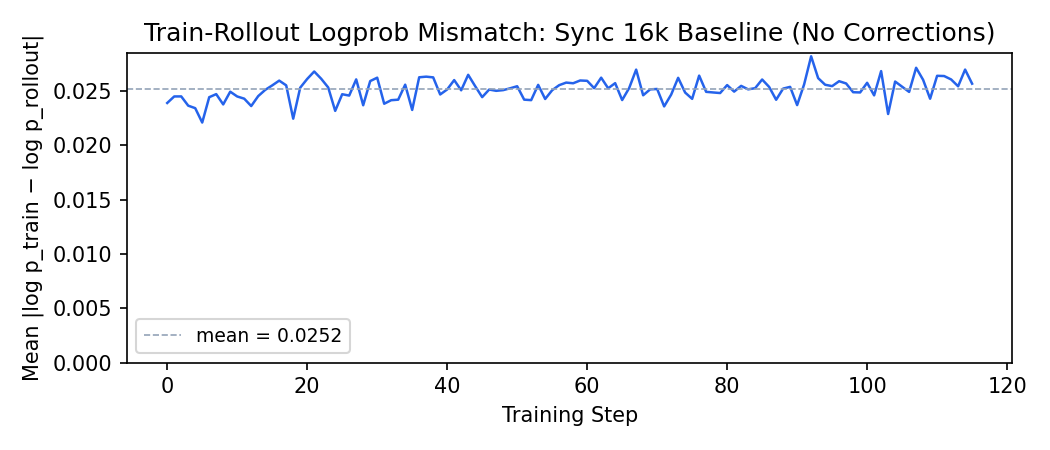
In the sync baseline, this metric sits at ~0.025 and stays flat throughout training — the mismatch is stable but non-negligible. This number becomes our reference point: any correction strategy in later stages needs to either reduce this gap (routing replay) or tolerate it gracefully (IS corrections). You can’t pick good clip bounds if you don’t know what “normal” looks like.
Stage 2: One-Step Async
The first thing we tried was simply switching to the train_async.py entrypoint — one-step off-policy, no corrections. The figure below shows our progression through four correction attempts:
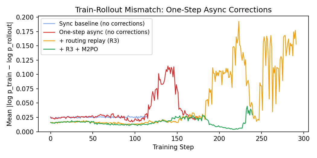
Without any corrections (red), the logprob diff blows up past 0.10 by step 130 — a 4× increase over the sync baseline. The natural fix for a sparse MoE is routing replay — replaying the rollout’s expert routing decisions during the training forward pass so both engines process the same tokens through the same experts. This is Source 4 in the off-policy corrections framework [7], and unlike the other sources, it’s best handled by elimination rather than correction.
The orange curve shows the effect: routing replay starts the logprob diff much lower (~0.016 vs ~0.025 — the routing component of the mismatch is gone), but the blowup is delayed, not prevented. The remaining mismatch from policy staleness and training-inference engine differences still accumulates and eventually diverges.
We then tried adding M2PO [2] on top of R3 — a staleness correction that masks tokens with high second-moment IS ratios. The green curve shows the result: it holds the logprob diff stable for much longer, but eventually diverges too around step 230.
Why did M2PO fail? M2PO computes the second moment $m_2 = (\log \pi_{\text{prox}} - \log \pi_{\text{behave}})^2$ for each token, sorts them, and masks the highest-variance tokens until the mean of the remaining falls below a threshold. The adaptive design is appealing — it masks as many tokens as needed to bring the mean under control.
The problem is that the M2 distribution in our setting is extremely heavy-tailed. At the onset of instability (step ~130), we added p90/p99 percentile logging and saw:
| Percentile | $m_2$ value | $\lvert\delta\rvert$ | Interpretation |
|---|---|---|---|
| p50 | ~3e-7 | ~0.0005 | Median token: negligible staleness |
| p99 | ~0.015 | ~0.12 | 99th percentile: mild staleness |
| max | ~1.0 | ~1.0 | Tiny fraction (<0.01%): extreme |
Five orders of magnitude between the median and the max. The extreme tokens are real and damaging, but they’re so rare that they barely move the mean. Meanwhile the M2PO mask rate stayed at exactly zero through the entire run — the mean never crossed the threshold.
No threshold setting fixes this for heavy-tailed distributions:
- Too high (e.g., 0.04): mean is well below → no masking ever triggers.
- At the boundary (e.g., 0.001): mean hovers right at the threshold → masking is unstable, often $k=0$.
- Too low (e.g., 1e-5): would need to mask >50% of tokens (since p50 > 1e-5) to drag the mean below threshold — catastrophic data loss.
We also tried a per-token hard cutoff (--m2-max-cutoff 0.1) to directly mask any token with $m_2 > 0.1$. The figure below shows the tradeoff: the max cutoff (purple) keeps the logprob diff under control, but raw reward drops sharply and never recovers. The original M2PO (green) maintains reward longer but eventually diverges. Neither mode solves the problem — aggressive masking throws away too much gradient signal from the hardest, most informative tokens.
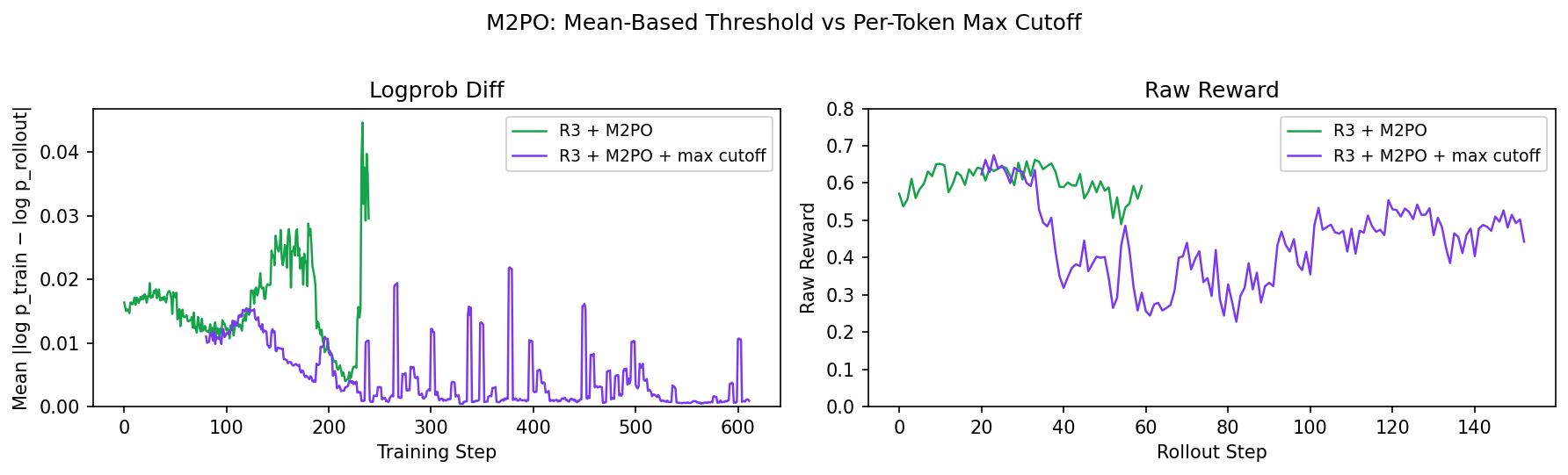
This points to a deeper limitation of masking-based corrections: they remove the most extreme outlier tokens but apply zero correction to surviving tokens, treating them as on-policy. With long sequences, the vast majority of tokens are moderately stale — not extreme enough to trigger any mask, but stale enough to accumulate uncorrected gradient noise. The damage comes from the mass of slightly-off tokens, not from a few extreme ones. And if you lower the mask threshold enough to catch those, you end up discarding most of your data.
What we needed was not just masking outliers, but actively reweighting the moderately stale tokens.
From M2PO to DPPO/TIS: Reweighting Instead of Masking
This led us to DPPO (Decoupled PPO), introduced in AReaL [3]. The key idea: in standard async PPO, the ratio $\pi_\theta / \pi_{\text{behav}}$ conflates two things — the policy update and the off-policy correction. DPPO decouples them by decomposing it as:
\[\frac{\pi_\theta}{\pi_{\text{behav}}} = \underbrace{\frac{\pi_\theta}{\pi_{\text{prox}}}}_{\text{clipped (trust region)}} \times \underbrace{\frac{\pi_{\text{prox}}}{\pi_{\text{behav}}}}_{\text{unclipped (reweighting)}}\]where $\pi_{\text{prox}}$ is a recent checkpoint that serves as the trust region center. Only $\pi_\theta / \pi_{\text{prox}}$ gets PPO-clipped; $\pi_{\text{prox}} / \pi_{\text{behav}}$ is kept as an unclipped multiplicative IS weight for off-policy correction.
For our first implementation, we unknowingly simplified this: the slime codebase labeled the inference log-probs as “old log probs,” so we ended up with a single combined ratio $\frac{\pi_\theta^{\text{Megatron}}(y_t)}{\pi_{\theta_{\text{old}}}^{\text{SGLang}}(y_t)}$ that lumps staleness and engine mismatch together, with a one-sided cap at 5.0 (adopted from the AReaL codebase, which adds this cap even though the paper doesn’t). Only later did we realize that accessing the true proximal policy (a separate checkpoint of the training weights at rollout time) required the --keep-old-actor flag — which led us to the proper decomposition. In this form, it’s equivalent to TIS with a one-sided cap — tokens with extreme upward ratios are zeroed out, while everything else gets reweighted proportionally.
The key difference from M2PO: every surviving token gets corrected proportionally to how off-policy it is, rather than being treated as on-policy. The moderately stale tokens that M2PO ignores are exactly the ones that benefit from reweighting.
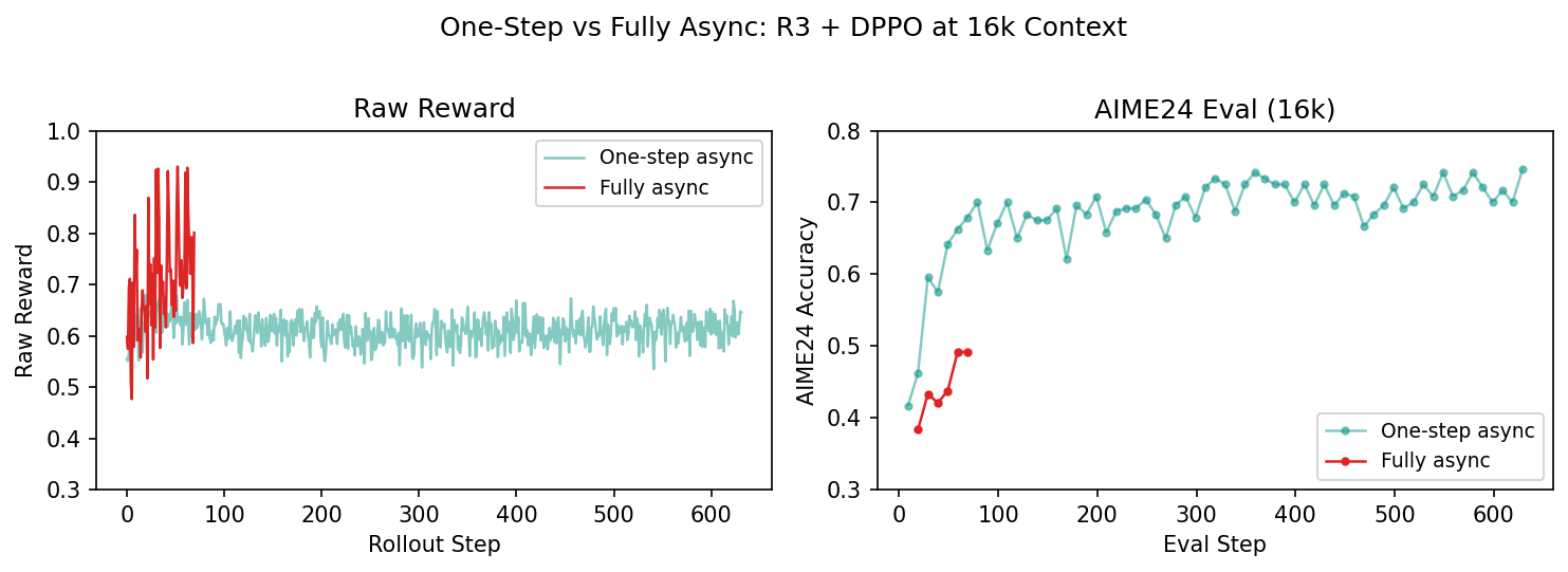
The decomposition into three independent ratios (CompIS) came later, once we moved to fully async and needed finer-grained control. But even this single-ratio version gave us our first stable async run:
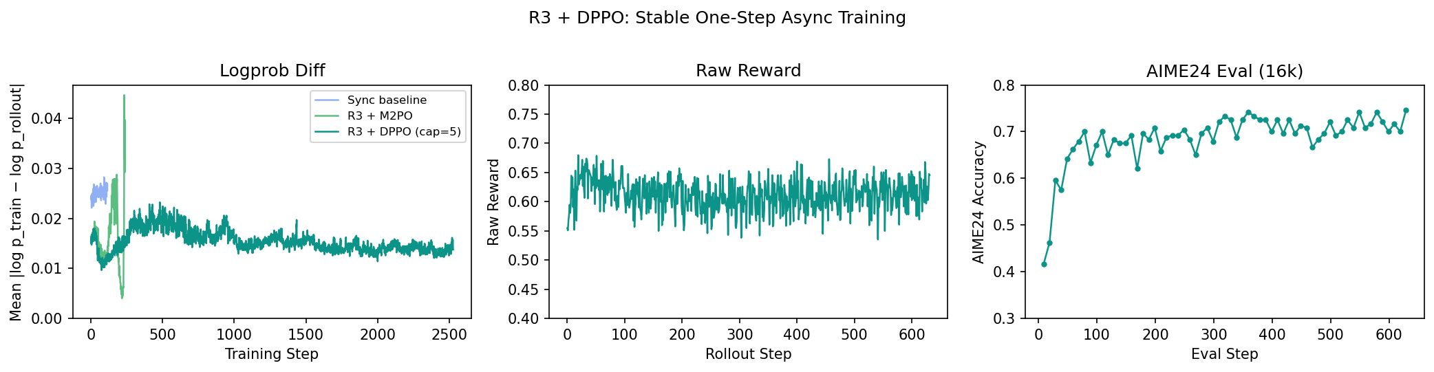
The logprob diff stays flat throughout training — no divergence. Raw reward is stable, and AIME24 eval under 16k context climbs steadily from ~0.42 to ~0.74.
From DPPO to CompIS: Decomposing the IS Ratio
With a working single-ratio DPPO, we went back to double-check the AReaL paper and discovered a discrepancy: the original actually decomposes the behavioral IS weight into two separate ratios (staleness and engine mismatch), while we had lumped them into one. This sent us down the analysis that became the companion post [7] — where we identified five independent sources of distribution mismatch and realized that each source has qualitatively different characteristics, meaning different correction strategies (cap, clip, hard rejection) could be applied flexibly per source.
This led to CompIS (“compass”) — a composable IS correction framework using a 3-ratio decomposition with routing replay handling Source 4 separately:
| Ratio | Source | Numerator | Denominator | Always present? |
|---|---|---|---|---|
| $r_1$ | Within-step drift | $\pi_\theta(y_t)$ | $\pi_{\theta_k}^{\text{Meg}}(y_t)$ | Yes (standard PPO) |
| $r_2$ | Engine mismatch | $\pi_{\theta_j}^{\text{Meg}}(y_t)$ | $\pi_{\theta_j}^{\text{SGL}}(y_t)$ | Yes (disaggregated) |
| $r_3$ | Staleness | $\pi_{\theta_k}^{\text{Meg}}(y_t)$ | $\pi_{\theta_j}^{\text{Meg}}(y_t)$ | Only when $k \neq j$ |
Where $\theta_j$ = weights at rollout time, $\theta_k$ = weights at training time, Meg = Megatron forward pass, SGL = SGLang forward pass.
Source 1 ($r_1$) is always corrected by PPO’s standard clip:
\[L^{\text{PPO}} = \min\left(r_1 \hat{A}, \text{clip}(r_1, 1-\varepsilon, 1+\varepsilon) \hat{A}\right)\]Sources 2 and 3 are applied as multiplicative IS weights on the PPO loss, each with its own configurable correction method:
# From loss.py — CompIS 3-ratio decomposition
# Source 1 (within-step drift): PPO clip already applied above

# Source 3 (staleness): Megatron(π_k) / Megatron(π_j)
s_weight, loss_masks, ... = compute_is_correction(
    numerator_log_probs=old_log_probs,        # Megatron(π_k)
    denominator_log_probs=old_actor_log_probs, # Megatron(π_j)
    method=args.staleness_correction_method,   # cap, clip, icepop, none
)
pg_loss = pg_loss * s_weight

# Source 2 (engine mismatch): Megatron(π_j) / SGLang(π_j)
e_weight, loss_masks, ... = compute_is_correction(
    numerator_log_probs=old_actor_log_probs,   # Megatron(π_j)
    denominator_log_probs=rollout_log_probs,    # SGLang(π_j)
    method=args.engine_correction_method,
)
pg_loss = pg_loss * e_weight
We implemented four correction methods that can be assigned to each source independently:
| Method | Behavior | Use case |
|---|---|---|
cap | Zero out tokens with ratio > threshold | One-sided rejection for extreme upward spikes |
clip | Clamp ratio to $[\ell, u]$ (TIS-style) | Soft correction; all tokens contribute |
icepop | Zero out tokens outside $[\ell, u]$ | Hard two-sided rejection for localized instability |
none | Raw ratio, no correction | When you want to measure but not correct |
Staleness is additionally bounded by --max-off-policy-steps: samples older than the threshold are discarded before training.
The full CompIS loss for a single token $y_t$:
\[\mathcal{L}_t = \underbrace{\min\!\left(\frac{\pi_\theta(y_t)}{\pi_{\theta_k}^{\text{Meg}}(y_t)}\hat{A},\; \text{clip}\!\left(\frac{\pi_\theta(y_t)}{\pi_{\theta_k}^{\text{Meg}}(y_t)}, 1\!\pm\!\varepsilon\right)\hat{A}\right)}_{\text{Source 1: PPO clip (within-step drift)}} \;\times\; \underbrace{f_s\!\left(\frac{\pi_{\theta_k}^{\text{Meg}}(y_t)}{\pi_{\theta_j}^{\text{Meg}}(y_t)}\right)}_{\text{Source 3: staleness}} \;\times\; \underbrace{f_e\!\left(\frac{\pi_{\theta_j}^{\text{Meg}}(y_t)}{\pi_{\theta_j}^{\text{SGL}}(y_t)}\right)}_{\text{Source 2: engine}}\]where $f_s$ and $f_e$ are independently configured correction functions (cap, clip, icepop, or none).
With CompIS in place, we were ready to go fully async.
Stage 3: Fully Async Training
With R3 + DPPO working on one-step async, we turned on fully async — rollout workers running continuously, independent of the training loop. Samples can now arrive with staleness $k = 1, 2, \ldots$ training steps.
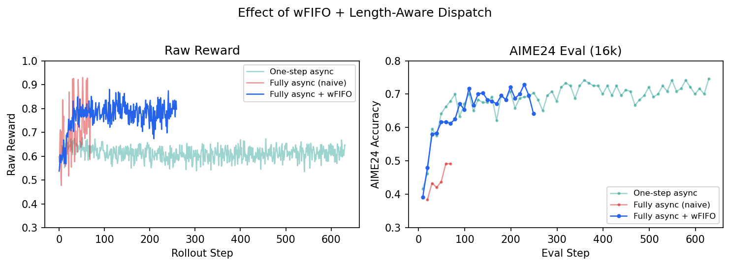
Training didn’t collapse — raw reward stayed positive and AIME24 eval improved. But comparing against our one-step async run revealed a problem:
Fully async has higher training reward but lower eval scores. This is the telltale sign of simplicity bias — the model is over-training on easy prompts that complete quickly, inflating the raw reward, while under-training on the hard prompts that actually matter for eval.
Engineering: The Simplicity Bias Problem
The mechanism is straightforward: easy prompts produce short responses that complete quickly, so they dominate the training batches in a naive FIFO drain.
We fixed this with a two-sided approach in the RolloutDataWorker, adapting ideas from FORGE [4] and SEER [5]:
Windowed FIFO drain. This directly addresses the difficulty distribution problem. Strict arrival order gives you simplicity bias; strict submission order blocks on the slowest sample and kills throughput. Our compromise is a sliding window over submission order — only groups within the window are eligible for consumption, and the window advances as head groups get consumed. This keeps the training batches close to the true prompt distribution without fully blocking on the long tail.
But windowed FIFO alone creates head-of-line stalling: the window can’t advance until its head groups complete, and if those happen to be hard/long prompts, everything waits. This is where length-aware dispatch comes in.
Length-aware dispatch. The key intuition is that response length is largely determined by the prompt itself — all $k$ samples in a group will have similar length. So we only need to measure one. The data worker sends the first sample of each prompt group as a “probe” at maximum priority. When the probe completes, its response length tells us how long the remaining $k-1$ samples will take, and we use it to prioritize them in the dispatch queue. Longer (harder) prompts get dispatched earlier, giving them a head start so they’re closer to completion when the window reaches them.
# Simplified from data_worker.py
def feed_queue(self, sampling_params):
    group = self.sampling.next_group()
    cached_len = self._prompt_metrics.get(prompt_key).expected_len

    if cached_len is unknown:
        # Probe: send sample[0] at maximum priority
        heappush(queue, (float("-inf"), seq, gid, 0, group[0]))
    else:
        # Cache hit: push all k samples at cached priority
        for i, s in enumerate(group):
            heappush(queue, (-cached_len, seq, gid, i, s))
Probe lengths are cached via EMA, so subsequent epochs skip the probe entirely and dispatch all $k$ samples immediately at the cached priority.
A bonus: the estimated lengths also improved load balancing in the slime router. Instead of balancing by number of jobs (which treats a 5k-token easy prompt the same as a 30k-token hard one), we balance by estimated work — distributing total expected tokens evenly across SGLang engines. This reduces stragglers and improves GPU utilization.
The two mechanisms work together: the windowed drain ensures training batches reflect the true prompt distribution, and length-aware dispatch reduces the stalling time at the window head by getting hard prompts started earlier.
Staleness rate-limiting. We also needed a hard bound on how far ahead rollout can get. The async worker caps in-flight groups at max_ahead = max_staleness × rollout_batch_size. When the limit is hit, rollout workers pause until training catches up.
The results confirm the fix. With wFIFO + length-aware dispatch, the raw reward comes back down from its inflated naive-async levels (the model is no longer over-training on easy prompts), and AIME24 eval recovers to match the one-step async reference:
Stage 4: Scaling Context — 16k → 32k → 64k
Looking at our 16k fully async runs, we noticed the raw reward was relatively high and the initial truncation rate was significant — many responses were hitting the 16k context ceiling. We switched to 32k rollout length with the Intellect3 Math prompts (19k harder problems) to give the model room to think longer.
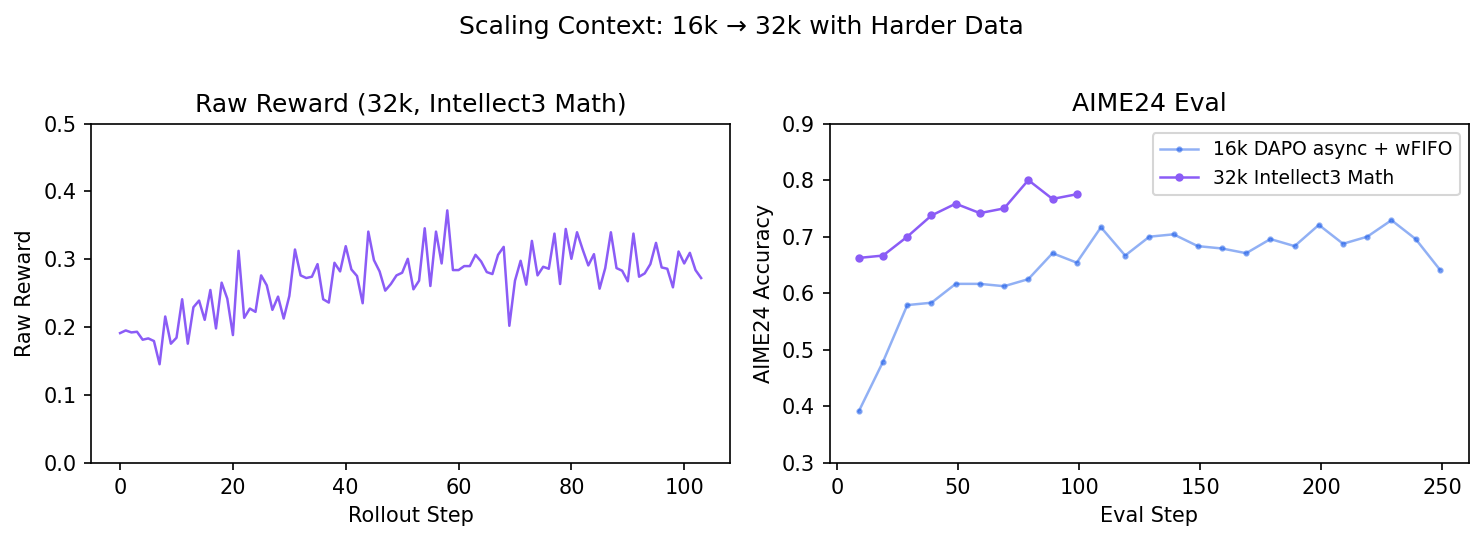
The 32k run was stable — raw reward is much lower (reflecting the harder prompt distribution), and AIME24 eval climbs steadily to ~0.80. But the low raw reward (~0.2–0.35) was a warning sign: around half the prompts in each batch (roughly 60 out of 128) were getting all-zero rewards — every sample in the group failed, so GRPO produces zero advantage and the prompt contributes nothing to the gradient. That’s a lot of wasted rollout compute.
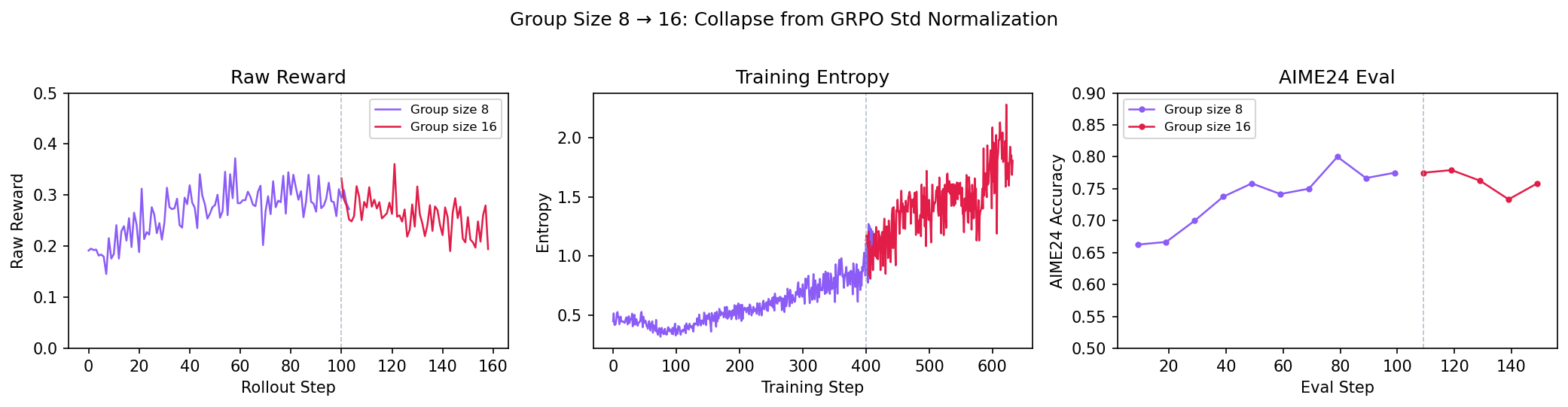
The natural fix was to increase the group size from 8 to 16 — more samples per prompt means more chances to get at least one success, so fewer prompts are wasted. But when we tried this, the model collapsed:
Failure cascade: raw reward decline → training entropy blowup → repetition rate increase → test performance collapse.
This was frustrating — a seemingly reasonable change (larger groups) made things much worse. But the fact that the collapse correlated precisely with the group size change pointed us straight to the culprit.
Fix 1: The GRPO Variance Normalization Trap
GRPO normalizes advantages by dividing by the per-group standard deviation:
\[\hat{A}_i = \frac{R_i - \bar{R}_{\text{group}}}{\sigma_{\text{group}}}\]Seems reasonable — normalize so the gradient scale is consistent across prompts. But with binary (0/1) outcome rewards, this normalization is actively working against you:
- Easy prompts (most samples pass): low variance → small $\sigma$ → inflated advantages. The model gets a strong signal to reinforce behavior it’s already good at.
- Hard prompts (most samples fail): low variance again → inflated advantages for rare successes, extreme penalties for failures.
- Mid-difficulty prompts (mixed pass/fail): high variance → large $\sigma$ → deflated advantages. These are exactly the prompts where the model is at the learning frontier, and the normalization is downweighting them.
In other words, GRPO’s normalization creates an inverted curriculum — it amplifies gradients from prompts the model has least to learn from, and suppresses gradients from prompts where learning is actually happening.
It gets worse with larger group sizes. More samples per prompt means the $\sigma$ estimates across prompts become more spread out, amplifying the distortion. So the fix that enables larger groups (removing the std normalization) is also more necessary at larger groups — a nice coincidence.
This was first identified by Dr.GRPO [6] and later adopted by DeepSeek V3.2. If you still want some form of normalization, REINFORCE++ offers a middle ground: it normalizes by global variance across the entire batch rather than per-group. The global estimate is stable enough that it doesn’t distort the difficulty distribution.
When normalization is needed: from our earlier work on process reward implementation, we found that mixing reward signals at different scales (e.g., process rewards + outcome rewards) does require normalization to prevent one signal from dominating. That’s the use case GRPO’s per-group std was designed for. But with pure binary outcome rewards, the scale is already fixed — there’s nothing to normalize, and the per-group std just introduces harmful difficulty reweighting.
Scaling to 64k
With the normalization fix (and group size 16), we moved to 64k context. The reward decline and entropy blowup came back:
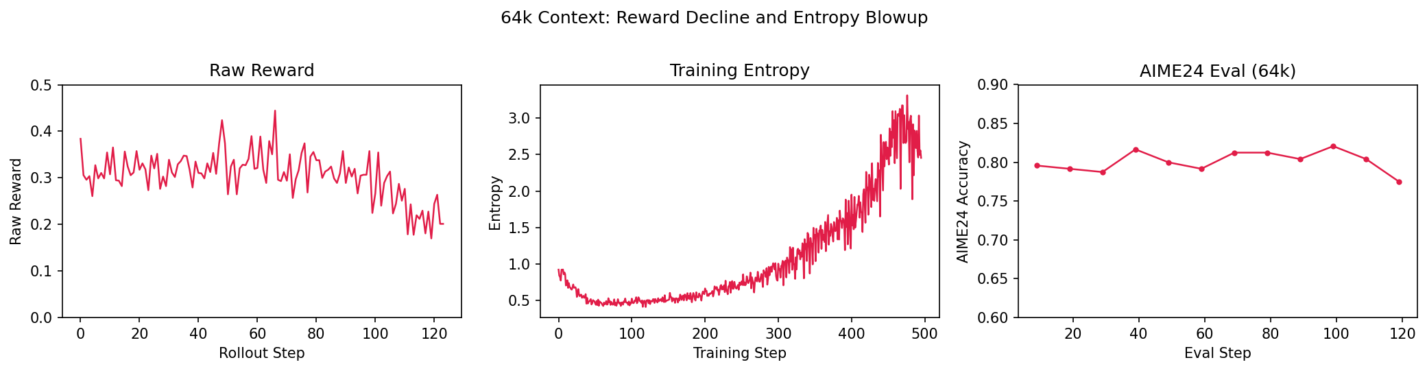
Our first hypothesis was that the data was simply too hard — the reward signal was too noisy to learn from. We tried mixing in easier data to provide denser reward, but it didn’t fix the downward trend in raw reward. The problem was somewhere in the training dynamics, not the data difficulty.
Fix 2: Two-Sided IS Ratio Bounds
Looking at the per-source IS diagnostics, we spotted the issue. The engine mismatch IS weight mean (which should sit at 1.0) showed frequent downward spikes:
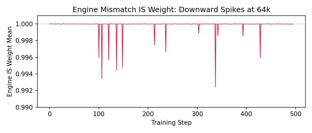
Our default CompIS configuration (following the AReaL codebase) only applied a one-sided cap on the staleness ratio and did not correct the engine mismatch ratio. At 16k and 32k this was fine — the engine mismatch was small enough to ignore. At 64k with hard data, these downward spikes became frequent enough to matter: a near-zero IS weight effectively zeroes out the gradient for that token, and when enough tokens are affected in the same batch, the update becomes noisy.
We switched to two-sided bounds, using ICEPoP-style token-level hard rejection: tokens with IS ratios outside $[\ell, u]$ are masked out, everything else contributes normally. This preserves the vast majority of each sequence’s gradient signal while catching outliers in both directions.
Fix 3: The Batch Size–Freshness Tradeoff
The standard recipe is 4 PPO mini-epochs over each batch of data. In synchronous training, this is fine — the data is on-policy at the start and drifts a little by epoch 4. In fully async training, the data is already stale when it arrives, and 4 epochs of additional within-batch drift make it worse.
We reduced mini-epochs from 4 → 1 and set the batch size to 1/4 of the original. An interesting side effect: with only 1 epoch, the PPO clip term effectively never activates — the policy hasn’t drifted enough within a single epoch for clipping to matter. This suggests that the “clip-higher” trick from DAPO (raising $\varepsilon$ to loosen the trust region) may be too aggressive for async RL, where the data is already off-policy before the first epoch begins. For MoE models specifically, reducing to 1 epoch has another benefit: within-batch gradient updates can shift routing decisions, which fights against the routing replay we worked so hard to set up. Fewer epochs means less routing drift within each batch.
| Config | Batch (prompts) | Epochs | Step time | Steps to cover same data |
|---|---|---|---|---|
| Original | $B$ | 4 | 1200s | 1 |
| Revised | $B/4$ | 1 | 330s | 4 |
Wall-clock for the same data: $4 \times 330\text{s} = 1320\text{s}$ vs. $1200\text{s}$ — only ~10% overhead. The extra cost comes from weight sync: each step transfers updated weights to the inference engines, and with 4× more steps, that sync happens 4× more often. But sync is a small fraction of total step time.
What surprised us was how much stability improved. It’s tempting to conclude that batch size and off-policy corrections are substitutes — that you can brute-force through variance with large batches instead of correcting it. But our experience suggests otherwise: larger batches can mask instability and give seemingly better upward trends early on, but they cannot sustain stable training without proper corrections. The underlying off-policy drift, routing mismatch, and advantage distortion are still there — large batches just average over them, delaying the collapse rather than preventing it.
The real benefit of smaller, fresher batches is that they complement the corrections: more frequent weight updates → fresher rollouts → less off-policy drift → corrections have less work to do. It’s a virtuous cycle, but only if the corrections are in place first.
The Final 64k Run
With all three fixes in place — no std normalization, two-sided IS bounds, and 1-epoch smaller batches — we got stable training at 64k context:
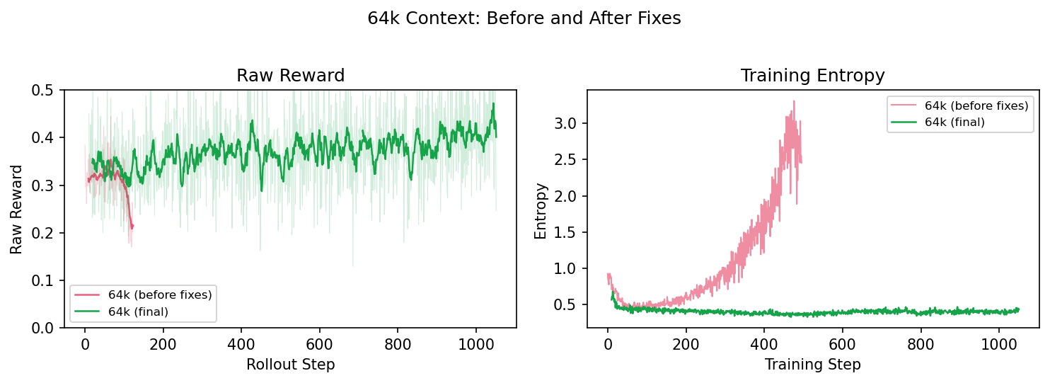
The contrast speaks for itself. The failed run’s entropy blows up and reward collapses; the final run holds steady across all metrics. We kept this run going for a week — the only interruption was a hardware NVLink failure, not a training instability. The recipe was stable.
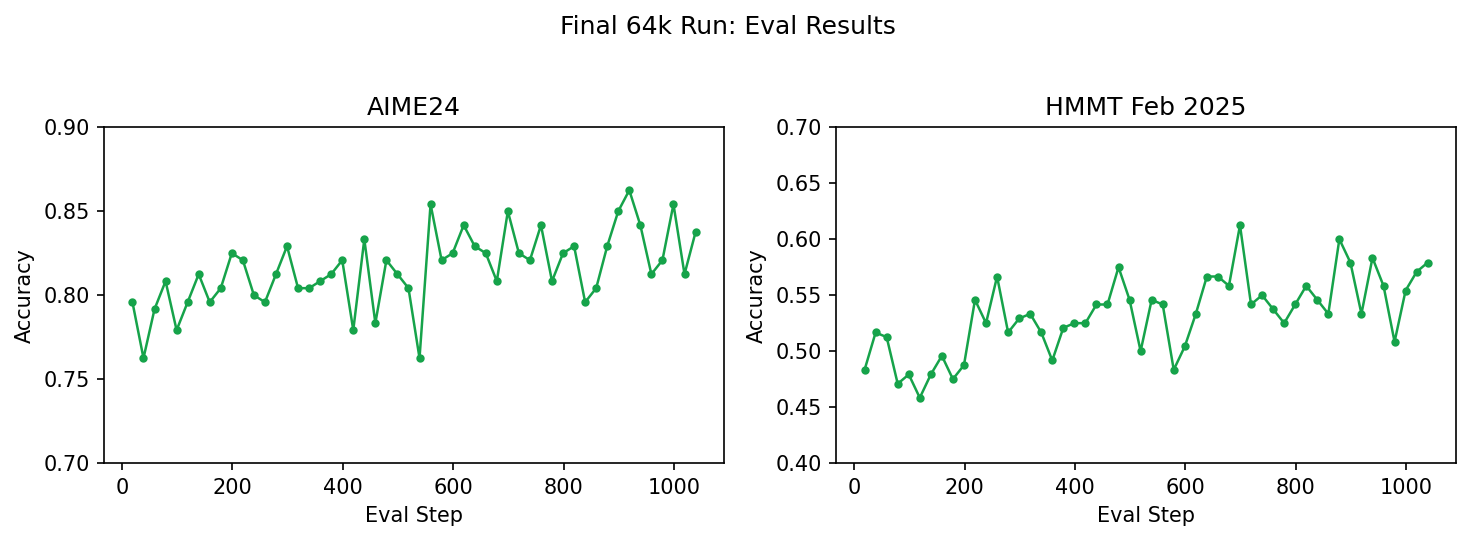
AIME24 holds steady around 0.82–0.85 (up from 0.80 at 32k), and HMMT Feb 2025 — a harder benchmark — trends upward from ~0.48 to ~0.58 over the course of the run.
Diagnostic Signals
Throughout this post, a handful of metrics consistently told us whether a run was headed for trouble — often before the reward curves did. Here’s what we learned to watch.
Train-rollout logprob absolute difference was our first line of defense. We tracked this from Stage 1 (the sync baseline at ~0.025) through every experiment. When it stayed flat, the system was healthy. When it diverged — as in the uncorrected one-step async run that blew up to 0.10 — something was fundamentally wrong with the IS correction or routing replay. This metric catches engine mismatch and staleness issues early.
Training entropy was the clearest early warning for model collapse. A mild decline or mild increase in entropy is both normal — the model is adjusting its confidence as it learns. What you’re looking for is a sudden upward spike: in every failed run — the group-16 collapse, the 64k failure — entropy blowup preceded the reward decline. A sharp spike means the policy is receiving contradictory gradient signals. We learned to intervene the moment entropy started spiking, before reward metrics confirmed the problem.
Raw reward vs eval divergence caught the simplicity bias. When training reward went up but AIME eval went down (as in our naive fully-async run), the model was over-fitting to easy prompts. This pattern is specific to async training with heterogeneous prompt difficulty.
Per-source IS ratio distributions are where CompIS’s decomposition really pays off for debugging. The engine weight mean plot at 64k (the downward spikes to ~0.992) directly led us to add two-sided IS bounds. Being able to see each correction source independently — staleness vs engine mismatch — meant we could diagnose which source was causing trouble without guessing.
Rollout log-prob trend is a useful leading indicator for model health more broadly. In failed runs, the model’s average log-probability of its own generations kept decreasing — the policy was becoming less confident in its own outputs, which preceded entropy blowup and repetition collapse. In stable runs, rollout log-prob slowly increased as the model converged. A consistent downward trend is a signal to intervene before reward metrics confirm the problem.
Percentile logging over mean logging (p50/p90/p99/max) taught us that mean-based diagnostics can hide heavy-tailed problems. The M2 mean looked benign while the max was 5 orders of magnitude higher. For any IS-based metric in long-context training, always check the tails, not just the mean.
What We Learned
Getting async RL right requires a combination of engineering and algorithmic fixes, and knowing which tool to reach for matters. Our overarching approach: fix what you can with engineering first — routing replay, data dispatch/drain, smaller fresher batches — to avoid being off-policy whenever possible. For the residual mismatch that engineering can’t eliminate, be principled about your algorithmic corrections — decompose IS ratios per-source, monitor clipping/capping rates, and don’t settle for heuristics that mask the problem. Watch diagnostic metrics that can alert you before eval starts to drop — entropy, logprob diff, per-source IS distributions. And start simple: get things working at 16k with one-step async before scaling to fully async at 64k. Fast iteration at a simpler setup teaches you more than long runs at a complex one.
Specific lessons
Eliminate before you correct. MoE routing replay was the single most impactful change early on — it removed an entire source of mismatch at the infrastructure level, making the remaining corrections tractable. Whenever a mismatch source can be eliminated (by replaying routing, syncing weights more frequently, or matching engine configurations), do that first.
Reweight, don't just mask. M2PO and other masking approaches failed because they treat surviving tokens as on-policy. With long sequences, the damage comes from the mass of moderately stale tokens, not a few extreme outliers. Continuous reweighting (as in DPPO/CompIS) corrects the entire distribution proportionally. Masking is a useful complement for extreme outliers, but it's not a substitute for reweighting.
Decompose your corrections. Lumping staleness and engine mismatch into a single IS ratio works at low staleness, but breaks down as you scale. The sources have qualitatively different distributions — separating them (CompIS) lets you tune each one independently and diagnose problems per-source.
Async training has its own data distribution problems. Simplicity bias — easy prompts dominating training batches — is not a staleness issue, and no amount of IS correction will fix it. It requires infrastructure-level fixes (windowed FIFO, length-aware dispatch) that are orthogonal to the algorithmic corrections.
GRPO's variance normalization is counterproductive with sparse binary rewards. This is easy to miss because it looks like a reasonable default. With 0/1 outcome rewards, per-group std normalization creates an inverted curriculum that gets worse with larger group sizes. Remove it, or use global normalization (REINFORCE++) instead.
Smaller, fresher batches complement corrections — they don't replace them. Large batches can mask instability by averaging over off-policy drift, but the underlying problems remain. With proper IS decomposition and routing replay in place, you can use 4× smaller batches at only ~10% wall-clock overhead, and the freshness benefit creates a virtuous cycle: more frequent weight updates → less drift → corrections have less work to do.
Limitations. Everything in this post is single-turn math RL: one prompt, one response, a binary reward. Real agent training adds layers of complexity we haven’t tackled — multi-turn trajectories where environment interactions introduce non-policy tokens into the conditioning context, reward models that add their own noise and drift, environment setup latency that further skews the async data distribution, and tool-call trajectories where standard IS ratios don’t cleanly apply (this is Source 5 in [7]). The principles here — eliminate before correcting, decompose your IS ratios, watch the diagnostics — should transfer, but the specifics will need revisiting.
References
[1] THUDM. “slime: Scalable LLM Inference and Megatron Engine.” GitHub.
[2] Xie, S., et al. “Prosperity before Collapse: How Far Can Off-Policy RL Reach with Stale Data on LLMs?” arXiv preprint arXiv:2510.01161 (2025). (M2PO)
[3] Mei, J., et al. “AReaL: An End-to-End Reinforcement Learning Framework for LLM Reasoning.” arXiv preprint arXiv:2505.24298 (2025). (DPPO)
[4] MiniMax-AI. “FORGE: A Scalable Agent RL Framework and Algorithm.” HuggingFace blog (2025). (Windowed FIFO)
[5] Qin, R., et al. “Seer: Online Context Learning for Fast Synchronous LLM Reinforcement Learning.” arXiv preprint arXiv:2511.14617 (2025). (Length-aware dispatch)
[6] Liu, Z., et al. “Dr.GRPO: Removing Variance Normalization in Group Relative Policy Optimization.” arXiv preprint arXiv:2503.20783 (2025).
[7] Off-Policy Corrections in LLM RL Training — Companion post: the five sources of distribution mismatch.