Optimizing Pass@k as Reweighting Prompts
Work in progress. This post is still being revised and this is an early preview.
In What’s in Pass@K?, we looked at what pass@k measures when it is used to evaluate a model. For a problem with pass rate $p$, the chance that a single sample is correct, pass@k is $1-(1-p)^k$. Improvements on easy problems barely move pass@k, and improvements on hard problems show up clearly.
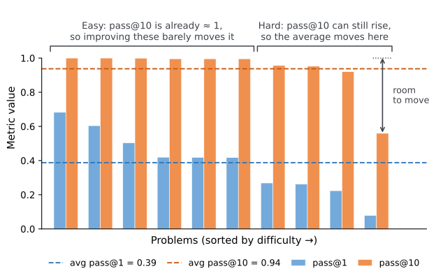
Figure 1 (annotated version of the figure in the previous post): pass@1 (blue) and pass@10 (orange) for 10 problems, sorted from easiest (left) to hardest (right). How much a problem’s pass@10 moves when its $p$ improves is the derivative $k(1-p)^{k-1}$: at k = 10, about 4.7 for the hardest problem ($p \approx 0.08$) and under 0.001 for the easiest ($p \approx 0.68$).
The same view says how to train for pass@k.
There is no need to compute pass@k at training time. Reweight the samples instead. Every sample keeps its own reward, and its gradient is weighted by how much pass@k would move if its prompt improved.
The gradient of pass@k with respect to the model’s parameters is
\[\nabla\, \text{pass@}k = k(1-p)^{k-1}\, \nabla p .\]Here $\nabla p$ is the gradient that ordinary RL with a binary reward follows, the pass@1 gradient. Optimizing pass@k is therefore pass@1 training with each prompt’s gradient multiplied by $k(1-p)^{k-1}$.
Once pass@k is written as a weight on prompts, two questions follow:
What should the weight be? The weight $k(1-p)^{k-1}$ depends on $p$, which we don’t know. Each prompt’s weight has to come from an estimate of $p$ from the rollouts, or an estimator that never needs $p$ at all.
Where do we apply the weight? It can scale each prompt’s gradient, through the reward or the loss. It can also decide what gets sampled: how often a prompt is drawn and how many rollouts it gets. Resampling is also reweighting, since drawing a prompt twice as often has, in expectation, the same effect as doubling its gradient.
Several recent papers answer parts of these questions: MaxRL [1], Reinforce-Ada [2], PKPO [3] and Never Give Up [4]. We put them in one frame and fill in a few gaps between them.
Part I. What Should the Weight Be?
1. Pass@k’s Weight
Averaged over the prompts in a training set, each with its own pass rate $p_x$, the gradient from the opening becomes
\[\nabla\, \mathbb{E}_x\big[\text{pass@}k(x)\big] = \mathbb{E}_x\big[\,w_k(p_x)\,\nabla p_x\,\big], \qquad w_k(p) = k(1-p)^{k-1}.\]At $k = 1$ the weight is 1 on every prompt, which is ordinary RL. For larger $k$ it starts at $k$ for $p = 0$ and falls faster the larger $k$ is (Figure 2, left): at $k = 8$, a prompt with $p = 0.1$ counts about 60 times as much as one with $p = 0.5$. Over a batch, the weight moves onto fewer and harder prompts as $k$ grows (Figure 2, right). At $k = 64$ the hardest tenth of the prompts carries 99% of it, and the rollouts spent on the rest barely move the model. Section 5 comes back to that cost.
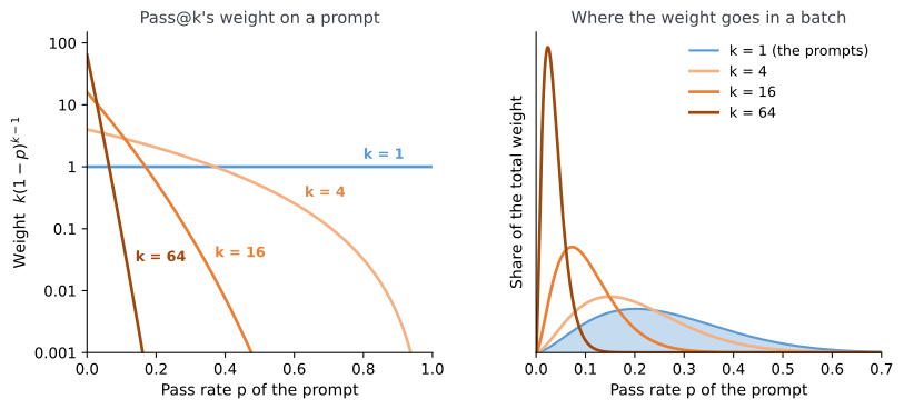
Figure 2. Left: pass@k’s weight on a prompt with pass rate $p$, for k = 1, 4, 16 and 64. Right: the share of the total weight carried by prompts of each pass rate, for a batch drawn from the illustrative difficulty distribution of the previous post (shaded; Beta(2.7, 7.7), mean pass rate 0.26).
The weight is largest at $p = 0$, where it cannot act. If all $G$ rollouts in a prompt’s group fail, its gradient estimate is zero, and no weight changes that. The chance of at least one success is pass@G itself: about 8% for $p = 0.01$ and $G = 8$. Only more samples help such a prompt (Section 5). The weight also depends on the pass rate, which we don’t know (Section 2).
2. Getting the Weight per Prompt
Estimating pass@k for evaluation was most of the previous post, and its three tools carry over to estimating the weight in training.
The empirical estimate of pass@k. The previous post computed pass@k from $N$ samples, $c$ of them correct, with the unbiased estimator $1-\binom{N-c}{k}/\binom{N}{k}$. It also used the shortcut $1-(1-\hat p)^k$ with $\hat p = c/N$, which is fine for ranking checkpoints but biased. The weight has the same two options. The shortcut $k(1-\hat p)^{k-1}$ is biased, and it scales a gradient computed from the same rollouts as $\hat p$. The unbiased route is the same estimator: $w_k(p)$ is $k$ times the chance that $k-1$ samples all fail, and with $c$ correct out of a prompt’s $G$ rollouts, $\binom{G-c}{k-1}/\binom{G}{k-1}$ estimates that chance without bias. PKPO [3] builds each rollout’s reward from this estimate, computed on the rollout’s $G-1$ siblings so that it is independent of the rollout it scales, and its expected update is exactly $\nabla\,$pass@k (Section 4). As in evaluation, $k$ can’t exceed the number of samples.
A prior for $p$. The previous post fitted a Beta distribution to the pass rates across problems and computed expected pass@k from it, which is stabler than per-problem estimates from few samples. At training time a prior matters for another reason: deciding how often to draw a prompt, or how many rollouts to give it (Section 5), needs the weight before the prompt’s rollouts exist. Reinforce-Ada-Est [2] keeps decayed counts of each prompt’s successes and trials on top of a Beta prior, so a prompt with no success in the current step keeps a nonzero estimate. The paper’s alternative is a small value network that predicts the pass rate from the prompt. A Beta posterior also gives the expected weight in closed form, the same way the previous post got expected pass@k: for $p \sim \text{Beta}(a, b)$, $\mathbb{E}[k(1-p)^{k-1}] = k\,B(a, b+k-1)/B(a, b)$. Fitting the prior across prompts, as the previous post did, would pull each prompt’s noisy estimate toward the rest of the dataset (empirical Bayes). We haven’t tested this, and whether it helps probably depends on the data, for example on how often each prompt comes back.
Sampling until you find a pass. The previous post suggested growing $N$ on hard problems until one or two samples pass. At training time this is Reinforce-Ada-Seq [2], which samples a prompt until it has $m$ correct rollouts, and NGU [4], which keeps retrying an unsolved prompt, with some chance of giving up, until a rollout passes. The rule needs no estimate of $p$ up front: it takes $m/p$ samples on average, so hard prompts get more rollouts automatically (Section 5 shows which weight this implements). If $p$ is wanted afterwards, the natural estimate $m/N$ after $N$ samples runs high, because sampling stops right after a success: at $m = 1$ and $p = 0.05$ it averages about three times the true $p$. The unbiased estimate is $(m-1)/(N-1)$ [6], which needs $m \ge 2$, one reason to wait for two passes rather than one.
3. Other Weights
We build on pass@k’s weight, but it isn’t the only one, and the recipe you already run has its own. Any objective that averages a function of the pass rate, $\mathbb{E}_x[f(p_x)]$, has a gradient of the same form, with weight $f’(p)$. MaxRL [1] and Reinforce-Ada [2] use this to compare training objectives, and Figure 3 puts the main ones next to pass@k’s.
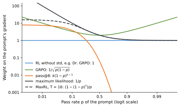
Figure 3. The weight each objective puts on a prompt’s gradient, following MaxRL’s comparison [1] with pass@8 added. The pass-rate axis is stretched at both ends (logit scale) to show the hard tail and GRPO’s rise near $p = 1$.
GRPO has an implicit weighting. GRPO divides each group’s advantages by the group’s standard deviation, and at the population level that makes its weight $1/\sqrt{p(1-p)}$ [1]. On hard prompts it grows like $1/\sqrt{p}$: faster than ordinary RL’s flat weight, but slower than maximum likelihood’s, below. It also rises again as $p \to 1$, so GRPO boosts nearly solved prompts too. Dropping the std division, as Dr. GRPO [5] does and as many current setups do (ours included), gives a weight of 1, plain pass@1. Compared with GRPO, that moves weight from both ends toward prompts of medium difficulty.1
Maximum likelihood maximizes \(\mathbb{E}_x[\log p_x]\), the log-probability of producing a correct answer, and its weight is $1/p$. It is a mix of every pass@k [1]: expanding $\log p = -\sum_{k\ge1}(1-p)^k/k$ gives
\[\frac{1}{p} = \sum_{k\ge 1} \frac{1}{k}\, w_k(p).\]Ordinary RL keeps only the $k = 1$ term. Like pass@k’s weight, $1/p$ is large on hard prompts, but it never falls below 1, because the $k = 1$ term is always in the sum. A single pass@k weight drops to nearly 0 once a prompt is solved some of the time, while $1/p$ keeps at least ordinary RL’s pressure on it. The conclusion comes back to this difference. MaxRL [1] truncates the sum at the group size $G$, which caps the weight near $G$ on the hardest prompts (dashed line in Figure 3).
Part II. Where to Apply the Weight?
The weight can scale each prompt’s gradient after sampling, or decide what gets sampled. In expectation the two are the same. If prompts are drawn from $q(x) \propto D(x)\,w(p_x)$ instead of the dataset distribution $D$,
\[\mathbb{E}_{x\sim D}\big[\,w(p_x)\,\nabla p_x\,\big] = Z\;\mathbb{E}_{x\sim q}\big[\,\nabla p_x\,\big], \qquad Z = \mathbb{E}_{x\sim D}\big[w(p_x)\big],\]and the constant $Z$ folds into the learning rate. Reinforce-Ada calls these explicit and implicit weighting [2]. What differs is the cost. Weighting in the gradient pays for every prompt’s rollouts and then scales most of them toward zero; weighting in the sampling spends rollouts where the weight is. Only the sampling can help a prompt the model has never solved, since a weight multiplies a gradient that is zero.
| Where the weight enters | Examples | Needs $\hat p$ before sampling | Rollouts on near-zero-weight prompts | Helps never-solved prompts |
|---|---|---|---|---|
| Reward or loss | PKPO, Pass@k Training, MaxRL | No | Paid for | No |
| How often a prompt is drawn | Sampling by $w(\hat p)$ | Yes | Mostly avoided | Through more draws |
| Rollouts per prompt | NGU, Reinforce-Ada | No when sampling until a pass; yes when sizes are set in advance | Cut early | Yes |
Table 1. The three places for the weight. All three have the same expected gradient up to a constant; they differ in what they cost and in what they need to know.
4. In the Gradient
After sampling, the weight can scale each rollout’s reward or each prompt’s loss. The two differ only in the order of the computation, before or after the advantage, and they have the same trade-offs.
- Pass@k Training [7] started from the direct approach: split a prompt’s rollouts into blocks of $k$ and give every rollout in a block the block’s best reward. The $k$ rollouts then share one reward, which is what the previous post called inefficient, and the paper itself moves on to averaging over all subsets of $k$ rollouts, which gives each rollout its own advantage.
PKPO [3] does the same average and derives rewards whose expected update is exactly $\nabla\,$pass@k for any $k \le G$. Its reward for rollout $i$ can be written as
\[s_i = \frac{k}{G}\Big[\, r_i\,\hat f_{-i} \;+\; \big(1-\hat f_{-i}\big) \Big], \qquad \hat f_{-i} = \binom{G-1-c_{-i}}{k-1}\Big/\binom{G-1}{k-1},\]where $r_i \in \lbrace 0, 1 \rbrace$ is its correctness and $c_{-i}$ the number of correct siblings. $\hat f_{-i}$ is the estimator for the chance that $k-1$ samples all fail, an unbiased estimate of $(1-p)^{k-1}$. So the first term is the rollout’s own reward times an estimate of pass@k’s weight, and the second depends only on the siblings, which makes it a baseline that averages to zero. PKPO is the callout’s recipe, done through the reward.
- MaxRL [1] applies the maximum-likelihood weight through the loss, also without forming $\hat p$. It averages the gradient over the correct rollouts only, dividing by the number of successes instead of the number of rollouts, and it keeps more of its training prompts solved at least once than GRPO does.
Either way, two limits remain. A prompt whose rollouts all fail gets no gradient, however large its weight [2]. Every prompt also still costs its full group of rollouts, even when its weight is near zero.
5. In the Sampling
Extra samples for a prompt can come as more draws or as a bigger group. For the same total, the two are equivalent in expectation when the loss averages over samples and the baseline leaves each sample out, since every sample then contributes the same expected gradient wherever it sits. The exception is a loss with per-group statistics: under MaxRL, which divides by each group’s number of passes, more draws add weight, while a bigger group mostly cuts variance and raises the cap on the weight (Section 3).
How often a prompt is drawn. Drawing prompts in proportion to $w(\hat p_x)$ matches the gradient route in expectation and spends the budget where the weight is. It needs the weight before sampling, so it needs a prior or a running estimate for each prompt (Section 2). Those have their own problems: estimates go stale, new prompts have no history, and a prompt estimated as solved is drawn so rarely that its estimate is slow to update.
How many rollouts it gets. For a prompt the model has never solved, what matters is the total number of samples, since it gives no gradient until one of them passes. Group sizes can be set before sampling from a running estimate. Reinforce-Ada [2], which uses the maximum-likelihood weight $1/p$ (Section 3), does this in its Ada-Est variant: rollouts in proportion to $1/\sqrt{\hat p}$, and the other $1/\sqrt{\hat p}$ in the gradient, for $1/p$ in total. Otherwise the group size is decided during sampling, by sampling until a pass.
Retrying within the step.
- Sampling until a pass (Section 2) sets that number during sampling, and it implements a weight without computing one. Summing the per-sample policy gradients of a prompt sampled until its first pass, capped at $T$ samples, gives in expectation $\big(1-(1-p)^T\big)\,\nabla p\,/\,p$, which is MaxRL’s truncated gradient (Wald’s identity: whether sample $i$ is drawn depends only on the samples before it).
- Splitting the weight between sampling and the gradient: Reinforce-Ada’s Ada-Seq [2] samples until a prompt has $m$ passes, which takes $m/p$ samples on average and so applies the weight through the sampling. It then downsamples to a small group for the update, which drops that weight, and multiplies $1/\hat p$ back into the gradient to restore it.2
Sampling until a pass, as Ada-Seq does it, runs in rounds inside a training step: a prompt without a pass gets another round of rollouts, and the step can’t start until the last prompt is done. The hardest prompts decide how long that takes, so the retries create a long tail of rollout requests that holds up training; in Reinforce-Ada’s runs, Ada-Seq’s steps take 1.4 to 2.8 times as long as GRPO’s [2]. The alternative is to defer the retry: once we know a prompt needs more samples, it joins the next wave of rollout requests instead of getting a round of its own. This is a choice about how sampling is scheduled, not about synchronous versus asynchronous RL. A synchronous trainer, which waits for every rollout request in a batch to finish, can defer retries the same way.
Retrying within the step
Retrying in the next wave
Figure 4. The two ways to schedule retries, with the same synchronous trainer (schematic). Each box is one prompt’s group of rollouts. Top: a prompt with no pass gets more rounds inside its step, and the step waits for it. Bottom: it joins the next wave, so every step is one wave long, and the retried prompt trains with rollouts from an earlier step. In the same time, the top finishes one training step and the bottom two.
Retrying in the next wave.
NGU [4] works this way: a prompt that needs more samples goes back into the generator’s queue. It starts each prompt with a small group of $G$ rollouts and drops the prompt if all pass; if all fail, it samples another group with probability $p_{\text{NGU}}$ and gives up otherwise, repeating until one passes. It then trains on one group: the new rollouts plus the failed ones from the last few steps. A staleness gate drops older failures from the update, but their rewards still count toward the baseline.3
The group size $G$, $p_{\text{NGU}}$ and the gate’s age cutoff are hyperparameters; NGU’s GSM8K runs use $G = 4$, $p_{\text{NGU}} = 0.95$ and 4 steps. A prompt then gets $G/\big(1 - p_{\text{NGU}}(1-p)^G\big)$ samples on average: about $G/\text{pass@}G$ on moderately hard prompts, and $G/(1-p_{\text{NGU}})$ for prompts it never solves, 80 with the GSM8K settings.
Conclusion
Training for pass@k comes down to two choices: a weight on each prompt, and a place in the training loop to apply it. Pass@k’s own weight, $k(1-p)^{k-1}$, puts nearly all of it on prompts the model rarely solves, and any recipe can follow it without explicitly computing pass@k over groups of samples.
Which place fits depends on whether you have an estimate of $p$, and whether you are willing to spend more compute:
- No per-prompt history. Put the weight in the reward or the loss, with an estimator that never forms $\hat p$: PKPO for pass@k’s weight, MaxRL for maximum likelihood’s. Every prompt still costs its full group of rollouts.
- A running estimate of each prompt’s pass rate. Draw prompts in proportion to their weight, so the rollout budget goes where the weight is. The estimates go stale, and prompts with little history need a prior.
- Many prompts the model has never solved. No weight helps these; only more samples do. Sample until a pass, and send the retries to the next wave of rollout requests so the hardest prompts don’t hold up every step. The cost is that a retried prompt trains with older rollouts.
One question remains: is optimizing pass@k enough, when users mostly see pass@1? Does pass@1 always improve along with pass@k, do we need a schedule that moves training back to pass@1, or should we use maximum likelihood’s $1/p$, which mixes every pass@k?
References
[1] Tajwar, F., Zeng, G., et al. “Maximum Likelihood Reinforcement Learning.” February 2026.
[2] Xiong, W., Ye, C., Liao, B., et al. “Reinforce-Ada: An Adaptive Sampling Framework under Non-linear RL Objectives.” 2025.
[3] Walder, C., and Karkhanis, D. “Pass@K Policy Optimization: Solving Harder Reinforcement Learning Problems.” NeurIPS 2025.
[4] Noukhovitch, M., Ivison, H., Lambert, N., and Courville, A. “Learning to Solve Hard Problems in RL for LLMs by Never Giving Up.” September 2026.
[5] Liu, Z., Chen, C., Li, W., Qi, P., Pang, T., Du, C., Lee, W. S., and Lin, M. “Understanding R1-Zero-Like Training: A Critical Perspective.” COLM 2025.
[6] Haldane, J. B. S. “On a Method of Estimating Frequencies.” Biometrika 33(3), 222–225, 1945.
[7] Chen, Z., Qin, X., Wu, Y., Ling, Y., Ye, Q., Zhao, W. X., and Shi, G. “Pass@k Training for Adaptively Balancing Exploration and Exploitation of Large Reasoning Models.” 2025.
We believe std rescaling should only be used to match rewards of different scales, and should not be applied when all rewards are on a 0/1 scale. With 0/1 rewards, a group’s std is about $\sqrt{\hat p(1-\hat p)}$, a function of the pass rate alone, so dividing by it doesn’t fix a scale; it reweights prompts by difficulty. ↩
We read the downsampling as a workaround for the training stack, not part of the method. Sampling until $m$ passes gives each prompt a random number of samples, and the paper downsamples so that every update has a fixed shape and costs the same as GRPO with 4 rollouts per prompt. Training on all the samples would apply the weight through the sample count, as in the previous bullet, with no $1/\hat p$ to multiply back. ↩
Because sampling stops at the first pass, the gate only ever drops failures, so the kept rollouts over-represent passes, and a baseline computed on them alone would run high. NGU computes the baseline over every rollout the prompt has had, keeps each pass’s advantage at $1-\bar r$, and rescales the kept failures’ advantages so the group’s advantages still sum to zero; it calls this anchoring the positives. With 32 rollouts, one pass and 16 kept, the baseline is $1/32$, the pass gets $31/32$, and each of the 15 kept failures gets $-\tfrac{1}{32}\cdot\tfrac{31}{15}$ instead of $-\tfrac{1}{32}$. We read this as a reweighting: the kept failures are scaled by (all failures)/(kept failures), so they stand in for the stale ones that were dropped. ↩